
Part 10 · Module 6
Reporting Survival Analysis
Learn how to report time origins, event definitions, follow-up, Kaplan–Meier estimates, hazard ratios, assumptions, competing risks and publication-ready survival figures.
Learning outcomes
After completing this lecture, you should be able to:
- Report time origins, events, censoring and follow-up clearly.
- Present event counts, numbers at risk, survival probabilities and median survival.
- Report log-rank and Cox results with effect estimates and confidence intervals.
- Describe proportional-hazards checks and alternatives when violated.
- Report competing-risk estimands and cumulative incidence correctly.
- Prepare publication-ready survival tables, figures and reporting paragraphs.
Overview
A survival-analysis report should allow readers to reconstruct:
- who entered the analysis;
- when follow-up began;
- what event was counted;
- how censoring occurred;
- how much follow-up was available;
- how many events occurred;
- which survival and hazard estimands were reported;
- whether assumptions were assessed.
A Kaplan–Meier curve or hazard ratio alone is incomplete.
Reporting should follow the relevant study-design guideline, such as CONSORT 2025 for randomised trials [1] or STROBE for observational cohorts [2], together with statistical-reporting guidance.
Downloadable simulated dataset
The shared Part 10 dataset is entirely simulated and contains no real patient information. Download the participant-level CSV, consult the data dictionary and usage notes, or recreate it with the standalone R script.
The latent-time columns are included only to explain the simulation and would not all be observable in a real study. Reported analyses should use the observed time and status variables described in the data dictionary.
Why this matters
Common survival-reporting problems include:
- no time origin;
- unclear censoring rule;
- event counts omitted;
- median follow-up calculated naively;
- Kaplan–Meier curves without risk tables;
- hazard ratios described as risks;
- proportional hazards not assessed;
- medians reported when not reached;
- one minus Kaplan–Meier used for competing risks;
- curve tails interpreted after nearly everyone has left the risk set.
Transparent reporting is essential because the same numerical output can represent different endpoints and assumptions.
When to use this framework
Use the framework for:
- trial manuscripts;
- cohort studies;
- prognostic studies;
- competing-risk reports;
- theses;
- conference abstracts;
- evidence tables.
The level of detail may differ, but the endpoint definition and effect measure must remain explicit.
Research question and variables
The reporting framework applies to:
- the analysis population;
- time origin;
- observed event or competing-event type;
- censoring status;
- treatment or exposure group;
- adjustment variables;
- prespecified landmark times;
- survival, hazard or restricted-time estimands.
Every reported estimate should be traceable to one clearly defined endpoint and analysis population.
Data structure
A standard right-censored analysis commonly uses one participant-level row containing:
| Variable | Reporting role |
|---|---|
| Participant identifier | Confirms one record per independent unit |
| Time | Duration from the stated origin |
| Event status | Identifies event versus censoring |
| Group or exposure | Defines the primary comparison |
| Covariates | Defines adjusted-model interpretation |
| Event type | Distinguishes competing outcomes where relevant |
Start–stop data, recurrent events, delayed entry and time-dependent covariates require additional variables and explicit description.
Statistical assumptions
Methods reporting checklist
Endpoint
Report:
- time origin;
- event;
- time unit;
- censoring rule;
- delayed entry;
- recurrent or competing events.
Analysis population
State:
- randomised or eligible population;
- exclusions;
- participants analysed;
- event count;
- missing dates or covariates.
Descriptive analysis
Name:
- Kaplan–Meier estimator;
- confidence-interval method;
- landmark times;
- median-survival method;
- follow-up summary method.
Group comparison
State:
- log-rank type;
- weighting;
- stratification;
- sidedness.
Regression
State:
- model;
- predictors;
- units;
- reference categories;
- ties method;
- proportional-hazards assessment;
- non-linear or time-dependent effects;
- missing-covariate method.
Competing risks
State:
- event of interest;
- competing events;
- cumulative-incidence estimator;
- cause-specific or subdistribution model;
- interpretation.
Results reporting checklist
Report:
- participants per group;
- deaths or other events;
- censored counts;
- numbers at risk;
- median survival if estimable;
- survival at prespecified landmarks;
- effect estimate with 95% CI;
- log-rank result where relevant;
- assumption diagnostics;
- sensitivity analyses;
- competing-event incidence.
Data example
Essential survival-reporting values
simulated dataTable 1. Overall-survival summary
| Measure | Usual care | Intervention |
|---|---|---|
| Participants | 120 | 120 |
| Deaths | 80 | 64 |
| Censored | 40 | 56 |
| Median survival | 22.5 months | 28.0 months |
| 12-month survival | 71.7% | 84.2% |
| 24-month survival | 45.5% | 59.5% |
| 36-month survival | 30.1% | 43.3% |
Table 2. Adjusted Cox model
| Effect | Estimate | 95% CI | p-value |
|---|---|---|---|
| Intervention versus usual care HR | 0.65 | 0.47 to 0.91 | 0.011 |
Follow-up reporting
Median observed follow-up is not the same as the median of raw observed times, because participants with early events shorten the raw-time distribution.
The reverse Kaplan–Meier method treats censoring as the event for follow-up estimation.
reverse_followup <- survfit(
  Surv(
    overall_time,
    1 - overall_event
  ) ~ 1,
  data = survival_data
)

quantile(
  reverse_followup,
  probs = 0.5
)
In the simulated study, reverse Kaplan–Meier median follow-up is 36 months because administrative censoring is concentrated at the planned study end.
Also report the maximum or interquartile follow-up when informative.
Worked example
Worked reporting workflow in R
make_survival_data <- function(n = 240) {
  id <- seq_len(n)
  group_numeric <- as.integer(id %% 2 == 0)
  age <- 35 + ((7 * id) %% 41)
  stage3 <- as.integer(id %% 3 == 0)

  deterministic_uniform <- function(multiplier) {
    (((id * multiplier) %% 997) + 0.5) / 998
  }

  u_recurrence <- deterministic_uniform(37)
  u_nonrecurrence_death <- deterministic_uniform(73)
  u_postrecurrence_death <- deterministic_uniform(109)
  u_dropout <- deterministic_uniform(149)
  u_dropout_time <- deterministic_uniform(181)

  recurrence_rate <-
    0.035 *
    exp(
      log(0.55) * group_numeric +
      0.025 * (age - 55) +
      0.55 * stage3
    )

  nonrecurrence_death_rate <-
    0.010 *
    exp(
      log(0.85) * group_numeric +
      0.030 * (age - 55) +
      0.40 * stage3
    )

  postrecurrence_death_rate <-
    0.060 *
    exp(
      log(0.85) * group_numeric +
      0.020 * (age - 55) +
      0.25 * stage3
    )

  recurrence_time <-
    -log(u_recurrence) / recurrence_rate

  nonrecurrence_death_time <-
    -log(u_nonrecurrence_death) /
    nonrecurrence_death_rate

  postrecurrence_death_delay <-
    -log(u_postrecurrence_death) /
    postrecurrence_death_rate

  overall_death_time <- pmin(
    nonrecurrence_death_time,
    recurrence_time +
      postrecurrence_death_delay
  )

  dropout_time <- ifelse(
    u_dropout < 0.22,
    12 + 24 * u_dropout_time,
    Inf
  )

  censor_time <- pmin(
    36,
    dropout_time
  )

  overall_time <- pmin(
    overall_death_time,
    censor_time
  )

  overall_event <- as.integer(
    overall_death_time <= censor_time
  )

  competing_time <- pmin(
    recurrence_time,
    nonrecurrence_death_time,
    censor_time
  )

  competing_status <- ifelse(
    recurrence_time <=
      nonrecurrence_death_time &
      recurrence_time <= censor_time,
    1L,
    ifelse(
      nonrecurrence_death_time <
        recurrence_time &
        nonrecurrence_death_time <=
          censor_time,
      2L,
      0L
    )
  )

  data.frame(
    id = id,
    group_numeric = group_numeric,
    group = factor(
      group_numeric,
      levels = c(0, 1),
      labels = c(
        "Usual care",
        "Intervention"
      )
    ),
    age = age,
    stage3 = stage3,
    stage = factor(
      stage3,
      levels = c(0, 1),
      labels = c("Stage II", "Stage III")
    ),
    overall_time = overall_time,
    overall_event = overall_event,
    competing_time = competing_time,
    competing_status = competing_status
  )
}

survival_data <- make_survival_data()

library(survival)

km_fit <- survfit(
  Surv(
    overall_time,
    overall_event
  ) ~ group,
  data = survival_data,
  conf.type = "log-log"
)

logrank_fit <- survdiff(
  Surv(
    overall_time,
    overall_event
  ) ~ group,
  data = survival_data
)

survival_data$age10 <-
  (survival_data$age - 55) / 10

cox_fit <- coxph(
  Surv(
    overall_time,
    overall_event
  ) ~ group + age10 + stage,
  data = survival_data,
  ties = "efron",
  x = TRUE
)

ph_test <- cox.zph(
  cox_fit
)

landmark_summary <- summary(
  km_fit,
  times = c(12, 24, 36),
  extend = TRUE
)

cox_table <- exp(
  cbind(
    hazard_ratio = coef(cox_fit),
    confint(cox_fit)
  )
)

landmark_summary
cox_table
ph_test
Selected reporting values
Deaths: 144 / 240
Log-rank chi-square: 6.00, p = 0.014
Adjusted intervention HR: 0.654
95% CI: 0.470 to 0.909
Cox p-value: 0.011
Final manuscript tables and figures should be generated consistently from the same checked analysis objects.
Publication-ready survival figure
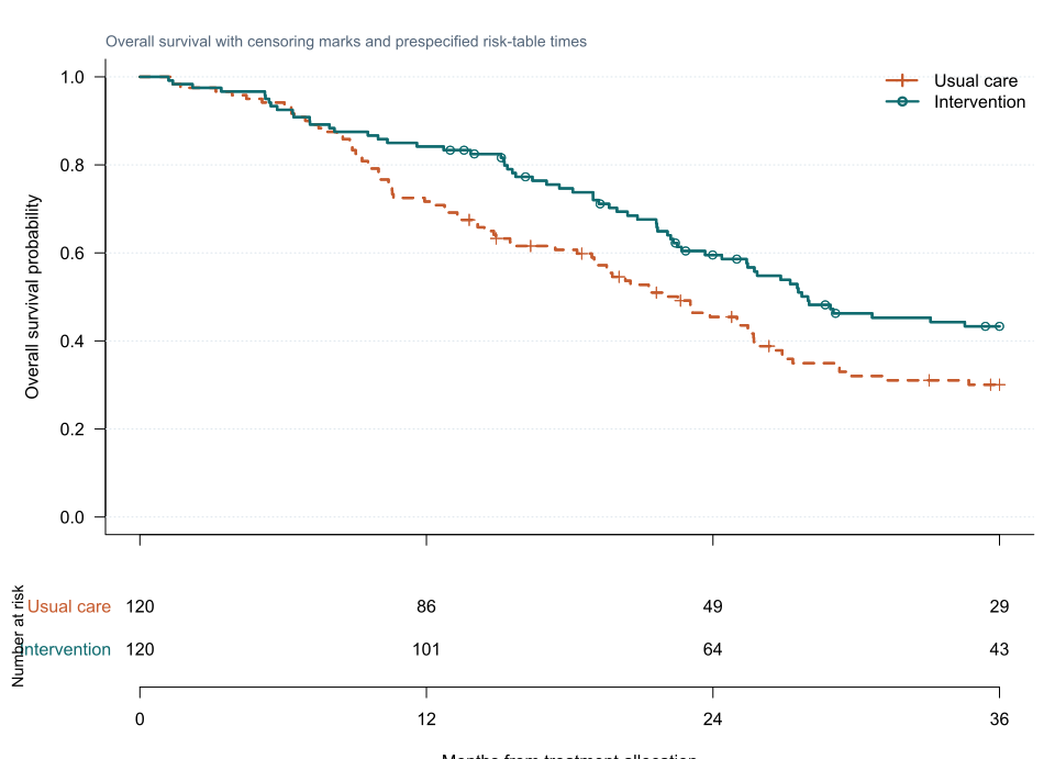
A strong survival figure should include:
- clear endpoint in the caption;
- time origin and units;
- group definitions;
- censoring marks where useful;
- numbers at risk;
- confidence intervals or separate reporting;
- sensible follow-up limit;
- accessibility without colour alone.
Reporting medians
Report the median and 95% CI when estimable.
If not reached, write:
Median survival was not reached during the observed follow-up.
Do not replace it with:
- mean observed follow-up;
- maximum time;
- a model extrapolation without disclosure.
Reporting hazard ratios
Always state:
- outcome event;
- reference group;
- adjustment variables;
- time scale;
- proportional-hazards assessment.
Avoid:
Intervention improved survival by 35%.
Prefer:
Intervention was associated with a 35% lower death hazard during follow-up, assuming proportional hazards.
Then provide absolute survival estimates.
Reporting non-proportional hazards
If proportional hazards is violated, do not report one ordinary HR without qualification.
Options include:
- interval-specific HRs;
- time-varying coefficient;
- landmark survival difference;
- restricted mean survival time;
- flexible parametric model.
Explain which estimand is primary.
Reporting competing risks
Report:
- event-of-interest CIF;
- competing-event CIF;
- event counts;
- cause-specific or subdistribution model;
- hazard type in the table heading.
Avoid:
Recurrence-free survival was 60%
when the analysis actually estimated recurrence cumulative incidence.
Tables and text
Use text for the primary message.
Use tables for:
- landmark survival;
- multiple predictors;
- competing-event estimates;
- sensitivity analyses.
Do not repeat every risk-table number in prose.
Interpreting survival results
Presenting the methods
Suggested reporting
For randomised trials, apply CONSORT 2025 [1]. For observational cohort studies, apply STROBE [2]. Use statistical-reporting principles such as SAMPL and good-practice recommendations for survival plots [3], [4]. Introductory survival-reporting principles are also summarised by Clark and colleagues [5].
Common mistakes
Knowledge check
What endpoint details must be reported?
Answer and reasoning
Time origin, event definition, time scale and censoring rule.
Why use reverse Kaplan–Meier for follow-up?
Answer and reasoning
It accounts for censoring appropriately rather than letting early events shorten the follow-up summary.
What must accompany a hazard ratio?
Answer and reasoning
The endpoint, reference, adjustment set, confidence interval, time scale and proportional-hazards assessment.
What should appear beneath a Kaplan–Meier plot?
Answer and reasoning
Numbers at risk at clinically meaningful times.
How should competing-risk results be labelled?
Answer and reasoning
By event type and estimand, such as recurrence cumulative incidence or cause-specific hazard ratio.
Key take-home messages
References
- Hopewell S, Chan AW, Collins GS, Hróbjartsson A, Moher D, Schulz KF, et al. CONSORT 2025 statement: updated guideline for reporting randomised trials. BMJ. 2025;389:e081123. https://doi.org/10.1136/bmj-2024-081123
- von Elm E, Altman DG, Egger M, Pocock SJ, Gøtzsche PC, Vandenbroucke JP, et al. The STROBE statement: guidelines for reporting observational studies. PLoS Med. 2007;4(10):e296. https://doi.org/10.1371/journal.pmed.0040296
- Lang TA, Altman DG. Basic statistical reporting for articles published in biomedical journals: the SAMPL guidelines. Int J Nurs Stud. 2015;52(1):5–9. https://doi.org/10.1016/j.ijnurstu.2014.09.006
- Pocock SJ, Clayton TC, Altman DG. Survival plots of time-to-event outcomes in clinical trials: good practice and pitfalls. Lancet. 2002;359(9318):1686–1689. https://doi.org/10.1016/S0140-6736(02)08594-X
- Clark TG, Bradburn MJ, Love SB, Altman DG. Survival analysis part I: basic concepts and first analyses. Br J Cancer. 2003;89(2):232–238. https://doi.org/10.1038/sj.bjc.6601118
These notes support learning and research planning and do not replace statistical consultation for a specific study.