
Part 6 · Module 7
Analysis of Covariance
Learn how analysis of covariance estimates adjusted group mean differences while accounting for a numerical baseline or prognostic covariate, with reproducible R output.
Learning outcomes
After completing this lecture, you should be able to:
- Explain analysis of covariance as a linear regression model.
- Estimate an adjusted treatment-group mean difference controlling for a baseline numerical covariate.
- Interpret the covariate coefficient, treatment coefficient and adjusted means.
- Assess linearity, influential observations and homogeneity of regression slopes.
- Distinguish baseline adjustment in randomised trials from confounder adjustment in observational studies.
- Use reproducible R code to fit, diagnose and report an ANCOVA model.
Overview
Analysis of covariance, abbreviated ANCOVA, is a linear regression model containing:
- a numerical outcome;
- one or more group indicators;
- and one or more numerical or categorical covariates.
In a randomised trial with a baseline measurement of the outcome, ANCOVA commonly estimates the treatment effect at follow-up after adjusting for baseline outcome. This approach is often more precise than an unadjusted follow-up comparison and generally preferable to comparing change scores [1], [2].
ANCOVA does not create randomisation or remove all confounding. In observational studies, adjustment requires a defensible causal or explanatory model, careful functional-form specification and adequate overlap [5].
Why this matters
Participants with higher baseline blood pressure tend to have higher follow-up blood pressure. Adjusting for baseline can explain predictable outcome variation and improve precision.
A simple follow-up t-test ignores this prognostic information. A change-score analysis subtracts baseline from follow-up but constrains the baseline coefficient implicitly and can be inefficient or misleading when baseline groups differ.
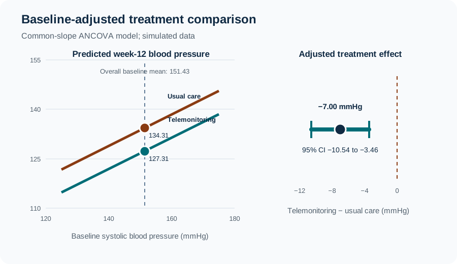
ANCOVA estimates the group contrast at a common baseline covariate value under the model.
When to use this method
Use ANCOVA when:
- the outcome is numerical;
- a group comparison is required;
- baseline outcome or another prognostic covariate is available;
- the adjusted mean difference is the intended estimand;
- observations are independent or dependence is modelled;
- and linear-model assumptions are sufficiently reasonable.
In randomised trials, prespecify adjustment variables in accordance with the protocol and applicable guidance [4]. Do not select them solely through univariable significance testing.
Research question and variables
The outcome is 12-week systolic blood pressure.
The exposure of interest is randomised group.
The covariate is baseline systolic blood pressure.
The treatment contrast is telemonitoring minus usual care.
The model assumes a common baseline–follow-up slope unless an interaction is included.
Data structure
ANCOVA data structure
simulated data| participant_id | group | sbp_baseline | sbp_week12 |
|---|---|---|---|
| U001 | Usual care | 146 | 137 |
| U002 | Usual care | 146 | 139 |
| T001 | Telemonitoring | 127 | 104 |
| T002 | Telemonitoring | 149 | 124 |
Note: The complete simulated dataset contains 80 participants.
The baseline measurement must occur before treatment can influence it. A post-randomisation variable should not be adjusted for casually because it may lie on the treatment pathway.
Statistical assumptions
Homogeneity of regression slopes
The standard model assumes the baseline slope is the same in both groups.
Assess this through:
- a scatter plot by group;
- clinical reasoning;
- and a treatment-by-baseline interaction model.
A non-significant interaction does not prove identical slopes, but a large or clinically meaningful interaction indicates that one adjusted group effect may be inadequate.
How the method works
For treatment coding for telemonitoring and for usual care:
Adjusted means can be calculated at the overall mean baseline value or standardised over the observed baseline distribution.
Worked example
Reproducible R analysis
ANCOVA is fitted as an ordinary linear model using base R’s lm() function [3].
trial <- data.frame(
  group = factor(
    rep(c("Usual care", "Telemonitoring"), each = 40),
    levels = c("Usual care", "Telemonitoring")
  ),
  sbp_baseline = c(
    146,146,138,150,146,169,147,150,157,146,129,150,163,145,144,144,177,158,153,157,
    156,134,153,152,147,159,157,160,150,151,130,143,152,138,148,146,148,141,151,164,
    127,149,165,168,155,160,136,141,167,149,143,164,157,142,161,146,155,138,145,134,
    162,155,140,172,157,146,148,149,161,128,157,169,162,153,148,160,168,160,167,155
  ),
  sbp_week12 = c(
    137,139,130,135,120,146,148,138,129,120,129,137,143,121,141,135,144,141,143,141,
    140,122,141,118,130,129,149,130,141,124,121,115,136,124,128,135,131,123,153,136,
    104,124,139,130,123,128,113,111,135,121,127,131,131,123,126,124,142,137,130,113,
    135,130,109,136,133,130,122,133,135,127,141,136,133,135,138,137,118,120,136,126
  )
)

# `lm()` fits the ANCOVA as a linear regression model [3]
fit <- lm(
  sbp_week12 ~ sbp_baseline + group,
  data = trial
)

summary(fit)
confint(fit)
anova(fit)
R coefficient output
                         Estimate Std. Error t value Pr(>|t|)
(Intercept)               62.2683    12.6282   4.931 4.60e-06
sbp_baseline               0.4758     0.0838   5.674 2.34e-07
groupTelemonitoring       -6.9999     1.7802  -3.932 0.000183
Confidence interval
groupTelemonitoring -10.5447 -3.4551Adjusted means at the overall baseline mean
reference_baseline <- mean(trial$sbp_baseline)

adjusted <- predict(
  fit,
  newdata = data.frame(
    sbp_baseline = reference_baseline,
    group = factor(
      c("Usual care", "Telemonitoring"),
      levels = levels(trial$group)
    )
  ),
  interval = "confidence"
)

adjusted
fit lwr upr
Usual care 134.31 131.80 136.82
Telemonitoring 127.31 124.80 129.83Model checks and verification
fit_interaction <- lm(
  sbp_week12 ~ sbp_baseline * group,
  data = trial
)

anova(fit, fit_interaction)

par(mfrow = c(2, 2))
plot(fit)
par(mfrow = c(1, 1))
Interpreting the output
Presenting the results
| Group | Baseline mean (SD) | Week-12 mean (SD) | Adjusted week-12 mean |
|---|---|---|---|
| Usual care | 149.9 (9.6) | 133.6 (9.5) | 134.3 |
| Telemonitoring | 153.0 (11.5) | 128.1 (9.1) | 127.3 |
Adjusted mean difference −7.0 mmHg (95% CI −10.5 to −3.5), .
Visualising the adjusted comparison
Suggested reporting
Randomisation and covariate adjustment MMed extension
In a randomised trial, baseline adjustment is used primarily to improve precision and account for chance baseline imbalance. It is not required to make treatment allocation unconfounded.
In observational studies, covariate adjustment aims to address confounding and requires stronger assumptions:
- relevant confounders measured adequately;
- correct functional form;
- positivity;
- no inappropriate control of mediators or colliders;
- and a clearly defined causal estimand.
Common mistakes
Knowledge check
What does the treatment coefficient estimate?
Answer and reasoning
It estimates the population mean follow-up difference between telemonitoring and usual care at the same baseline covariate value under the fitted model.
Why include baseline outcome?
Answer and reasoning
Baseline outcome is often strongly prognostic of follow-up, so adjustment can reduce residual variation and improve treatment-effect precision.
What is homogeneity of regression slopes?
Answer and reasoning
It is the assumption that the relationship between baseline and follow-up outcome is sufficiently similar across groups for one common slope and one adjusted treatment effect.
Should treatment adherence measured after randomisation be adjusted for routinely?
Answer and reasoning
No. It may be affected by treatment and lie on the causal pathway. Adjustment can change the estimand and introduce bias.
Does ANCOVA prove causality in an observational comparison?
Answer and reasoning
No. Causal interpretation additionally requires a defensible design and assumptions about confounding, measurement and model specification.
Key take-home messages
References
- Vickers AJ, Altman DG. Analysing controlled trials with baseline and follow up measurements. BMJ. 2001;323(7321):1123–1124. https://doi.org/10.1136/bmj.323.7321.1123
- Senn S. Change from baseline and analysis of covariance revisited. Stat Med. 2006;25(24):4334–4344. https://doi.org/10.1002/sim.2682
- R Core Team. Fitting linear models. R documentation, package stats version 4.6.1. Vienna: R Foundation for Statistical Computing; 2026. https://search.r-project.org/R/refmans/stats/html/lm.html
- European Medicines Agency. Guideline on adjustment for baseline covariates in clinical trials. EMA/CHMP/295050/2013. London: EMA; 2015. https://www.ema.europa.eu/en/adjustment-baseline-covariates-clinical-trials-scientific-guideline
- Harrell FE Jr. Regression modeling strategies. 2nd ed. Cham: Springer; 2015. https://doi.org/10.1007/978-3-319-19425-7
These notes support learning and research planning and do not replace statistical consultation for a specific study.