Why Repeated Observations Are Not Independent

Overview

Repeated observations from the same participant are usually more similar to one another than observations from different participants.

Examples include repeated blood pressure, daily pain scores, both eyes from one person, several lesions from one patient, and participants treated within the same clinic.

The rows in a dataset are therefore not automatically independent analytical units. The source of shared variation must be represented in the design, analysis and uncertainty estimates [1], [2].

Why this matters

If three measurements are recorded for each of 120 participants, the dataset has 360 rows but only 120 independent participants.

Treating all 360 rows as unrelated can:

• give participants with more records excessive weight;
• produce incorrect standard errors;
• distort confidence intervals and p-values;
• misrepresent effective sample size;
• create invalid sample-size calculations.

The distortion is not guaranteed to move every standard error in the same direction. Correlation can make between-participant effects less precise while making within-participant change contrasts more precise. The central problem is that the independent-row variance formula is wrong.

When to use this framework

Use the framework whenever observations are grouped naturally within participants, matched sets, families, clinics, schools, wards, readers or specimens.

Before choosing a model, identify the level at which units were independently sampled or allocated.

Research question and variables

The repeated outcome is systolic blood pressure.

Structural variables are:

• id: participant identifier;
• month: repeated time;
• group: usual care or telemonitoring;
• sbp: systolic blood pressure.

Time varies within participants. Group, age and sex are constant within participants.

Data structure

Long-format repeated data

simulated data

Table 1. First two participants

id	Group	Month	Systolic blood pressure
1	Usual care	0	160.5
1	Usual care	3	150.3
1	Usual care	6	148.5
2	Telemonitoring	0	163.0
2	Telemonitoring	3	150.2
2	Telemonitoring	6	143.7

Note: Three rows belong to each participant.

The long structure requires one row per participant-time observation and one correct participant identifier.

Statistical assumptions

Sources of dependence

Stable participant characteristics create shared variation across visits. Measurements close in time may also have serial correlation. The same device, observer or clinic can create further common effects.

How the method works

The intraclass correlation coefficient is:

For equal cluster size $m$, the common design-effect approximation is:

$$DE=1+(m-1)ICC$$

Worked example

Worked analysis in R

make_longitudinal_data <- function(n = 120) {
  records <- vector("list", n * 3)
  row_number <- 1

  for (participant_id in seq_len(n)) {
    group <- as.integer(participant_id %% 2 == 0)
    age <- 35 + ((7 * participant_id) %% 41)
    male <- as.integer(participant_id %% 3 == 0)

    random_intercept <-
      7 * sin(participant_id * 0.71) +
      3 * cos(participant_id * 0.19)

    random_slope <-
      0.45 * sin(participant_id * 0.37)

    for (month in c(0, 3, 6)) {
      residual <-
        3.5 * sin(participant_id * 1.13 + month * 0.91) +
        1.2 * cos(participant_id * 0.23 + month * 0.33)

      sbp <-
        151 +
        0.18 * (age - 55) +
        1.8 * male +
        random_intercept -
        1.5 * month -
        0.4 * group -
        0.75 * group * month +
        random_slope * month +
        residual

      records[[row_number]] <- data.frame(
        id = participant_id,
        group = group,
        age = age,
        male = male,
        month = month,
        sbp = sbp
      )

      row_number <- row_number + 1
    }
  }

  longitudinal <- do.call(rbind, records)

  longitudinal$group <- factor(
    longitudinal$group,
    levels = c(0, 1),
    labels = c("Usual care", "Telemonitoring")
  )

  longitudinal <- longitudinal[
    order(longitudinal$id, longitudinal$month),
  ]

  rownames(longitudinal) <- NULL
  longitudinal
}

longitudinal <- make_longitudinal_data()

wide <- reshape(
  longitudinal[c("id", "month", "sbp")],
  idvar = "id",
  timevar = "month",
  direction = "wide"
)

cor(
  wide[c("sbp.0", "sbp.3", "sbp.6")]
)

naive_model <- lm(
  sbp ~ group * month + age + male,
  data = longitudinal
)

clustered_vcov <- sandwich::vcovCL(
  naive_model,
  cluster = longitudinal$id,
  type = "HC1"
)

cbind(
  estimate = coef(naive_model),
  naive_se = sqrt(diag(vcov(naive_model))),
  clustered_se = sqrt(diag(clustered_vcov))
)

Selected analysis output

Baseline–month 3 correlation   0.696
Baseline–month 6 correlation   0.854
Month 3–month 6 correlation   0.735

Cluster-robust variance is shown only to demonstrate dependence-aware uncertainty. It does not replace a fully specified longitudinal model. Generalised estimating equations provide one formal population-averaged approach for correlated outcomes [3].

Visualising repeated dependence

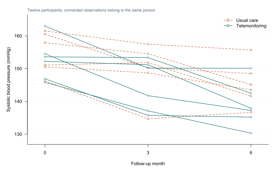
Interpreting the output

Presenting the results

Suggested reporting

Report participant count, observation count, visits per participant, missing visits, correlation or covariance approach, model interpretation and any small-cluster correction.

Longitudinal texts emphasise separating the mean structure from within-unit covariance [1], [2].

Common mistakes

Knowledge check

Why are 360 rows not 360 independent participants?

Answer and reasoning

They arise from 120 people measured three times. Observations from the same person share characteristics and measurement history.

What does an ICC near zero imply?

Answer and reasoning

Under the stated model, little residual variance is attributable to clusters. It does not prove complete independence.

Why can within-person effects be more precise?

Answer and reasoning

Stable participant characteristics can be controlled implicitly when change is estimated within the same people.

Is a cluster-robust SE always sufficient?

Answer and reasoning

No. It corrects selected variance calculations but does not define trajectories or solve missing-data problems.

What variable is essential in long repeated data?

Answer and reasoning

A correct participant or cluster identifier linking observations from the same independent unit.

Key take-home messages

References

1. Diggle PJ, Heagerty P, Liang KY, Zeger SL. Analysis of longitudinal data. 2nd ed. Oxford: Oxford University Press; 2002. https://doi.org/10.1093/oso/9780198524847.001.0001
2. Fitzmaurice GM, Laird NM, Ware JH. Applied longitudinal analysis. 2nd ed. Hoboken (NJ): Wiley; 2011.
3. Liang KY, Zeger SL. Longitudinal data analysis using generalized linear models. Biometrika. 1986;73(1):13–22. https://doi.org/10.1093/biomet/73.1.13