Multinomial Logistic Regression

Overview

Multinomial logistic regression models a nominal outcome with three or more unordered categories.

Examples include:

• discharged home, transferred or died;
• no complication, infection or bleeding;
• treatment A, B or C selected;
• stable, controlled or adverse clinical status.

One category is chosen as the reference. The model estimates one logit equation for every non-reference category versus that reference.

Why this matters

A nominal outcome should not be converted into arbitrary numerical scores. Separate binary models can also produce incoherent probabilities that do not sum to one.

Multinomial regression estimates the category probabilities jointly, but each coefficient is category-specific and must be labelled carefully.

When to use this method

Use multinomial logistic regression when:

• the outcome has at least three unordered categories;
• one outcome is observed per independent participant;
• category-specific comparisons answer the question;
• and cell information supports the number of parameters.

Use ordinal regression when the categories have a defensible order and a cumulative model is appropriate.

Research question and variables

For outcome category $j$ and reference category 0:

Data structure

Simulated outcome distribution

simulated data

Outcome category	Count
Stable	27
Controlled	100
Adverse	53

Note: The categories are nominal for this teaching example.

Statistical assumptions

How the method works

With three categories and four predictors, the model estimates two sets of four slopes plus two intercepts.

Predicted category probabilities are obtained by exponentiating all category linear predictors and normalising them so that probabilities sum to one.

Choosing the reference category

The reference outcome should be clinically meaningful and sufficiently frequent. Changing it alters coefficient presentation but not fitted category probabilities.

When controlled status is the main clinical target, the investigator may prefer controlled as the reference to compare stable and adverse outcomes directly with it. The choice should be specified before inspecting coefficients.

Parameter count

For $J$ outcome categories and $p$ predictor slopes, a baseline-category model estimates:

$$(J-1)(p+1)$$

parameters including category-specific intercepts. A four-level categorical predictor adds three slopes to every non-reference outcome equation.

Sparse outcome categories therefore create substantial instability even when the overall sample size appears large.

Predicted probabilities

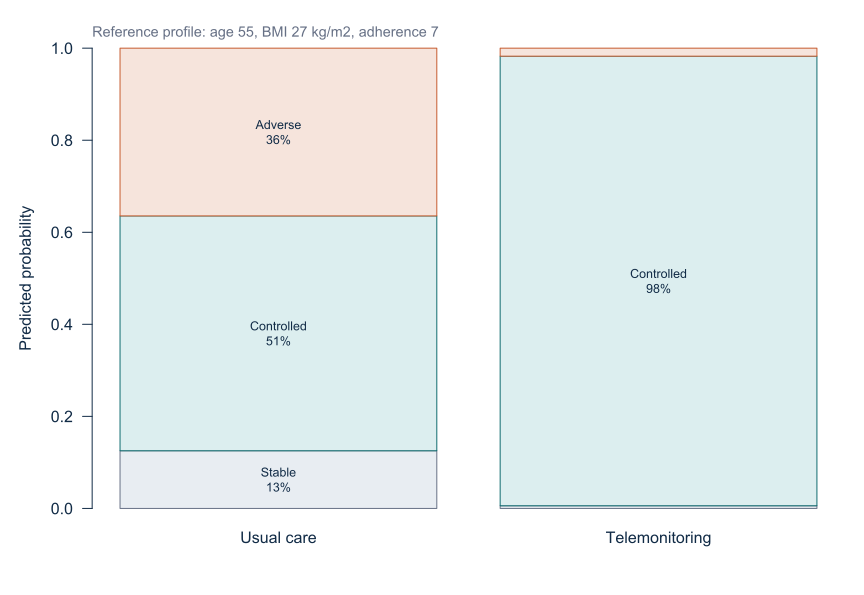
For each participant, the exponentiated linear predictors are converted to probabilities that sum to one. These probabilities often provide the clearest interpretation.

A predictor can increase the relative odds of one category versus the reference while another category probability also changes because all probabilities are linked. Report several representative profiles or standardised category probabilities.

Comparing non-reference categories

The coefficient for controlled versus stable and the coefficient for adverse versus stable can be subtracted to obtain adverse versus controlled on the log-relative-odds scale.

Its standard error must include the covariance between the two estimated coefficients. Simply dividing the two separately reported p-values or comparing their significance is invalid.

Independence of irrelevant alternatives

The independence-of-irrelevant-alternatives assumption concerns the relative odds between outcome categories. It may be questionable when categories represent closely related alternatives, such as discharge to two similar facilities.

Clinical outcome categories are often generated by an underlying sequence or hierarchy. In such settings, nested logit, continuation-ratio or multistate approaches may better represent the process.

Model assessment

Assessment includes:

• category-specific residual or influence patterns;
• functional forms for continuous predictors;
• sparse-cell and separation review;
• calibration of each category probability;
• discrimination summaries appropriate to multiple categories;
• validation in new data when prediction is intended.

An overall likelihood-ratio test can show that a predictor contributes somewhere in the outcome distribution but does not identify the specific category contrast.

Nominal versus ordinal modelling

An ordinal model is more parsimonious because it imposes an ordered structure and often one common slope. Multinomial modelling is more flexible but uses more parameters.

Do not choose the multinomial model merely because it makes fewer assumptions. The categories’ clinical meaning and available information should determine the model.

Worked example

Reproducible R analysis

make_hypertension_data <- function(n = 180) {
  set.seed(4583)
  i <- seq_len(n)

  data <- data.frame(
    participant_id = sprintf("H%03d", i),
    age = round(runif(n, 30, 80)),
    male = rbinom(n, 1, 0.5),
    bmi = pmin(pmax(round(rnorm(n, 27, 3.5), 1), 18), 40),
    physical_activity = round(runif(n, 2, 7), 1),
    telemonitoring = rbinom(n, 1, 0.5)
  )

  data$adherence <- 4 + runif(n, 0, 5) -
    0.015 * (data$age - 55) + 0.4 * data$telemonitoring
  data$baseline_sbp <- 92 + 0.52 * data$age + 0.85 * data$bmi +
    2.8 * data$male - 1.3 * data$physical_activity + rnorm(n, 0, 4)
  data$followup_sbp <- 58 + 0.47 * data$baseline_sbp +
    0.10 * data$age + 0.52 * data$bmi - 2.0 * data$adherence +
    2.0 * data$male - 4.5 * data$telemonitoring -
    0.55 * data$telemonitoring * (data$bmi - 27) +
    0.006 * (data$age - 55)^2 + rnorm(n, 0, 5)

  data
}

hypertension <- make_hypertension_data()

i <- seq_len(nrow(hypertension))

utility_stable <- rep(0, nrow(hypertension))

utility_controlled <-
  0.9 * hypertension$telemonitoring +
  0.35 * (hypertension$adherence - 6) -
  0.035 * (hypertension$baseline_sbp - 140) +
  0.8 * sin(i * 0.91)

utility_adverse <-
  0.035 * (hypertension$age - 55) +
  0.09 * (hypertension$bmi - 27) -
  0.4 * hypertension$telemonitoring +
  0.8 * cos(i * 1.17)

utilities <- cbind(
  Stable = utility_stable,
  Controlled = utility_controlled,
  Adverse = utility_adverse
)

hypertension$status <- factor(
  colnames(utilities)[max.col(utilities, ties.method = "first")],
  levels = c("Stable", "Controlled", "Adverse")
)

fit <- nnet::multinom(
  status ~ telemonitoring + age + bmi + adherence,
  data = hypertension,
  Hess = TRUE,
  trace = FALSE
)

summary(fit)

coefficients <- coef(fit)
standard_errors <- summary(fit)$standard.errors
z_values <- coefficients / standard_errors
p_values <- 2 * pnorm(-abs(z_values))
relative_odds <- exp(coefficients)

relative_odds

Cleaned R output

Outcome contrast       Predictor        Coefficient   Relative odds ratio   p-value
Controlled vs stable   Telemonitoring      3.713             40.98          <0.001
Controlled vs stable   Age               -0.018              0.982           0.485
Controlled vs stable   BMI                0.053              1.055           0.605
Controlled vs stable   Adherence          1.302              3.68           <0.001
Adverse vs stable      Telemonitoring      0.018              1.02            0.985
Adverse vs stable      Age                0.097              1.102           <0.001
Adverse vs stable      BMI                0.277              1.319           0.015
Adverse vs stable      Adherence          0.587              1.80            0.050

The recommended nnet package provides multinom() for multinomial log-linear models [1], [2].

Interpreting the output

Presenting the results

Present every coefficient with its outcome contrast and include observed or predicted category probabilities.

Visualising predicted nominal outcomes

Suggested reporting

Independence of irrelevant alternatives MMed extension

The standard multinomial logit assumes that relative odds between two categories are unaffected by the presence or characteristics of other alternatives.

This may be implausible when outcome categories are close substitutes or hierarchically related. Alternative models may be required [3].

Common mistakes

Knowledge check

Why is stable status the reference category?

Answer and reasoning

It provides the denominator category for both modelled logits. Another reference could be chosen if a different contrast is clinically primary.

What does the telemonitoring relative OR of 40.98 compare?

Answer and reasoning

It compares controlled with stable status, conditional on the included predictors.

Does the adverse-versus-stable coefficient compare adverse with controlled?

Answer and reasoning

No. That requires a different reference category or an explicit contrast.

Why not code the categories 1, 2 and 3 and fit linear regression?

Answer and reasoning

The categories are unordered, and numerical coding would impose unsupported spacing and order.

What should accompany relative odds ratios?

Answer and reasoning

Observed and predicted category probabilities, reference definitions and confidence intervals.

Key take-home messages

References

1. Venables WN, Ripley BD. Modern applied statistics with S. 4th ed. New York: Springer; 2002. https://doi.org/10.1007/978-0-387-21706-2
2. Ripley B. nnet: feed-forward neural networks and multinomial log-linear models. R package version 7.3-20. 2025. https://doi.org/10.32614/CRAN.package.nnet
3. Agresti A. Categorical data analysis. 3rd ed. Hoboken (NJ): Wiley; 2013.