
Part 6 · Module 5
One-Way Analysis of Variance
Learn how to compare mean numerical outcomes across three or more independent groups using one-way ANOVA, planned contrasts, Tukey intervals and reproducible R output.
Learning outcomes
After completing this lecture, you should be able to:
- Explain the overall null hypothesis in a one-way analysis of variance.
- Distinguish between-group and within-group variation.
- Calculate and interpret the F statistic, effect-size measures and overall p-value.
- Use planned contrasts or multiplicity-adjusted pairwise comparisons after fitting the overall model.
- Assess independence, variance and residual assumptions.
- Use reproducible R code to fit, diagnose and report a one-way ANOVA.
Overview
One-way analysis of variance, abbreviated one-way ANOVA, compares the means of one numerical outcome across three or more independent groups defined by one categorical factor.
Examples include comparing:
- mean functional score across three rehabilitation programmes;
- mean haemoglobin concentration across four disease-severity groups;
- mean hospital stay across several surgical techniques; and
- mean laboratory yield across multiple preparation methods.
The overall ANOVA asks whether all population means are equal. If the overall null is rejected, the analysis does not identify automatically which groups differ. Planned contrasts or multiplicity-adjusted pairwise comparisons are then required.
ANOVA is a linear model. The F statistic compares variation explained by group membership with residual variation within groups.
Why this matters
Performing several ordinary two-sample t-tests across three or more groups inflates the probability of at least one false-positive conclusion.
For three groups there are three pairwise comparisons. For five groups there are ten. The analysis should therefore distinguish:
- the overall group question;
- prespecified scientific contrasts;
- exploratory pairwise comparisons;
- and multiplicity control.
A significant overall F test means that at least one population mean differs from another. It does not imply that every pair differs.
When to use this method
Use one-way ANOVA when:
- the outcome is numerical;
- one categorical factor defines three or more independent groups;
- one outcome value is observed per analytical unit;
- mean comparisons answer the question;
- and the linear-model assumptions are sufficiently reasonable.
Use another method when:
- observations are paired, repeated or clustered;
- two factors are central;
- baseline adjustment is required;
- the outcome is binary, ordinal or count;
- or a rank-based distributional contrast is the estimand.
Research question and variables
The outcome is physical-function score.
The explanatory factor is programme with three levels.
The population means are:
- : usual care;
- : standard rehabilitation;
- : enhanced rehabilitation.
The overall alternative is that at least one population mean differs.
The effect should also be described using:
- group mean differences;
- simultaneous confidence intervals;
- and an overall effect-size measure.
Data structure
Independent-group ANOVA structure
simulated data| participant_id | programme | function_score |
|---|---|---|
| U001 | Usual care | 81 |
| U002 | Usual care | 61 |
| S001 | Standard rehabilitation | 82 |
| S002 | Standard rehabilitation | 68 |
| E001 | Enhanced rehabilitation | 81 |
| E002 | Enhanced rehabilitation | 84 |
Note: The complete balanced dataset contains 72 participants.
Each participant appears once. Programme should be a factor with a prespecified reference and display order.
Statistical assumptions
Moderate non-normality is often less concerning in balanced groups of reasonable size than severe outliers or dependence.
If variances differ materially, Welch’s one-way test can be used with oneway.test(..., var.equal = FALSE) [2]. If covariate adjustment is required, use linear regression or ANCOVA rather than a simple one-way procedure.
How the method works
The total variability is partitioned into:
- between-group sum of squares;
- within-group or residual sum of squares.
A large F value indicates that group mean differences are large relative to within-group variation.
Effect-size measures
Eta squared is:
Omega squared adjusts partly for positive small-sample bias and is a useful supplementary ANOVA effect-size measure [6]:
These proportions do not replace pairwise differences in clinical units.
Worked example
Reproducible R analysis
Base R fits the balanced model with aov() and constructs Tukey family-wise intervals with TukeyHSD() [4], [5].
rehab <- data.frame(
  programme = factor(
    rep(c("Usual care", "Standard rehabilitation", "Enhanced rehabilitation"), each = 24),
    levels = c("Usual care", "Standard rehabilitation", "Enhanced rehabilitation")
  ),
  function_score = c(
    81, 61, 68, 71, 66, 66, 80, 67, 80, 69, 71, 76,
    78, 67, 77, 62, 77, 81, 63, 78, 53, 87, 75, 73,
    82, 68, 79, 72, 72, 75, 75, 79, 71, 79, 82, 73,
    83, 88, 80, 83, 74, 79, 83, 73, 74, 94, 76, 68,
    81, 84, 81, 95, 69, 104, 82, 90, 79, 82, 86, 90,
    81, 88, 88, 86, 87, 65, 83, 79, 92, 74, 70, 101
  )
)

# `aov()` fits the balanced one-way model [4]
fit <- aov(function_score ~ programme, data = rehab)

summary(fit)
# `TukeyHSD()` gives family-wise simultaneous intervals [5]
TukeyHSD(fit, "programme", conf.level = 0.95)
R ANOVA output
             Df Sum Sq Mean Sq F value   Pr(>F)
programme     2 1754.9   877.4   13.98 7.98e-06
Residuals    69 4329.8    62.8
R Tukey output
Standard rehabilitation-Usual care
 diff = 5.6250, lwr = 0.1476, upr = 11.1024, p adj = 0.0428

Enhanced rehabilitation-Usual care
 diff = 12.0833, lwr = 6.6059, upr = 17.5608, p adj = 0.000004

Enhanced rehabilitation-Standard rehabilitation
 diff = 6.4583, lwr = 0.9809, upr = 11.9358, p adj = 0.0168
Cleaned output and checks
aov_table <- summary(fit)[[1]]
ss_between <- aov_table["programme", "Sum Sq"]
ss_residual <- aov_table["Residuals", "Sum Sq"]
ms_residual <- aov_table["Residuals", "Mean Sq"]

eta_squared <- ss_between / (ss_between + ss_residual)
omega_squared <- (
  ss_between - 2 * ms_residual
) / (
  ss_between + ss_residual + ms_residual
)

aggregate(
  function_score ~ programme,
  data = rehab,
  FUN = function(x) c(n = length(x), mean = mean(x), sd = sd(x))
)

data.frame(
  F = aov_table["programme", "F value"],
  df1 = 2,
  df2 = 69,
  p_value = aov_table["programme", "Pr(>F)"],
  eta_squared = eta_squared,
  omega_squared = omega_squared
)
Interpreting the output
Presenting the results
| Programme | n | Mean (SD) |
|---|---|---|
| Usual care | 24 | 72.0 (8.0) |
| Standard rehabilitation | 24 | 77.6 (6.2) |
| Enhanced rehabilitation | 24 | 84.0 (9.2) |
Overall one-way ANOVA: , , .
Visualising the results
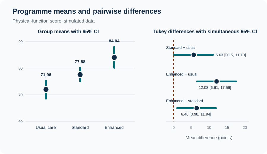
Suggested reporting
Welch ANOVA and regression modelling MMed extension
When group variances differ, Welch’s one-way test is often preferable to the conventional pooled-variance ANOVA.
oneway.test(
  function_score ~ programme,
  data = rehab,
  var.equal = FALSE
)
If group sizes are unequal, covariates are required or specific contrasts are primary, fit an explicit linear model and use contrast methods compatible with the design.
Common mistakes
Knowledge check
What does the overall ANOVA null hypothesis state?
Answer and reasoning
It states that all population group means are equal. Its rejection means at least one mean differs.
Why not run three unadjusted t-tests for three groups?
Answer and reasoning
The family contains several opportunities for false-positive findings. ANOVA and adjusted or prespecified contrasts provide a coherent error-control strategy.
What does the F ratio compare?
Answer and reasoning
It compares variability attributable to differences among group means with residual variability among participants within groups.
Does a significant F test identify which group is best?
Answer and reasoning
No. Group-specific estimates and planned or adjusted comparisons are required, together with clinical interpretation.
When is Welch's one-way test useful?
Answer and reasoning
It is useful when comparing independent means and the equal-population-variance assumption is doubtful, especially with unequal group sizes.
Key take-home messages
References
- Fisher RA. Statistical methods for research workers. Edinburgh: Oliver and Boyd; 1925.
- Welch BL. On the comparison of several mean values: an alternative approach. Biometrika. 1951;38(3–4):330–336. https://doi.org/10.1093/biomet/38.3-4.330
- Tukey JW. Comparing individual means in the analysis of variance. Biometrics. 1949;5(2):99–114. https://doi.org/10.2307/3001913
- R Core Team. Fit an analysis of variance model. R documentation, package stats version 4.6.1. Vienna: R Foundation for Statistical Computing; 2026. https://search.r-project.org/R/refmans/stats/html/aov.html
- R Core Team. Compute Tukey honest significant differences. R documentation, package stats version 4.6.1. Vienna: R Foundation for Statistical Computing; 2026. https://search.r-project.org/R/refmans/stats/html/TukeyHSD.html
- Lakens D. Calculating and reporting effect sizes to facilitate cumulative science: a practical primer for t-tests and ANOVAs. Front Psychol. 2013;4:863. https://doi.org/10.3389/fpsyg.2013.00863
These notes support learning and research planning and do not replace statistical consultation for a specific study.