Log-Rank Test

Overview

The log-rank test compares survival experience between two or more groups while accounting for right censoring.

At each event time, it compares:

• observed events in each group;
• expected events if groups had the same event hazard at that time.

These contributions are summed over follow-up.

The standard log-rank test gives equal weight to every event. It is most efficient for a persistent proportional-hazards-type difference, although the formal null concerns equality of survival experience rather than a specific constant hazard ratio [1].

Why this matters

A visible separation between Kaplan–Meier curves does not quantify whether the pattern is compatible with chance under the null model.

Conversely, a log-rank p-value does not show:

• how large the survival difference is;
• which landmark times matter;
• whether curves cross;
• whether the proportional-hazards assumption is plausible;
• whether adjustment is needed.

The test should accompany survival estimates and a clinically interpretable effect measure.

When to use this method

Use a log-rank test when:

• the endpoint is a right-censored time to one event;
• groups are independent;
• a global unadjusted comparison is required;
• censoring assumptions are plausible;
• event weighting across time is appropriate.

Use stratified log-rank methods when randomisation or analysis is stratified.

Use other estimands or weighted methods when clinically important effects are delayed, transient or crossing.

Research question and variables

The null hypothesis is:

$$H_0: S_I(t)=S_U(t) \text{ for all relevant }t$$

where $S_I(t)$ and $S_U(t)$ are intervention and usual-care survival functions.

The test uses:

• group;
• observed time;
• event indicator;
• changing risk sets.

Data structure

Risk-set contribution at one event time

simulated data

Suppose immediately before an event time:

Group	At risk	Observed deaths
Usual care	80	1
Intervention	90	0
Total	170	1

If hazards were equal, the expected intervention deaths would be:

$$1\times\frac{90}{170}=0.529$$

The intervention contribution to observed minus expected events is:

$$0-0.529=-0.529$$

A negative cumulative score for intervention indicates fewer deaths than expected under equal survival.

Statistical assumptions

How the method works

At event time $t_j$:

• $n_{1j}$ and $n_{0j}$ are group risk-set sizes;
• $d_j$ total events occur;
• $d_{1j}$ occur in group 1.

The expected group-1 event count is:

The total score is:

$$U= \sum_j(d_{1j}-E_{1j})$$

The test statistic is:

Worked example

Worked analysis in R

The survival package implements the log-rank test using survdiff() with rho = 0 [2].

make_survival_data <- function(n = 240) {
  id <- seq_len(n)
  group_numeric <- as.integer(id %% 2 == 0)
  age <- 35 + ((7 * id) %% 41)
  stage3 <- as.integer(id %% 3 == 0)

  deterministic_uniform <- function(multiplier) {
    (((id * multiplier) %% 997) + 0.5) / 998
  }

  u_recurrence <- deterministic_uniform(37)
  u_nonrecurrence_death <- deterministic_uniform(73)
  u_postrecurrence_death <- deterministic_uniform(109)
  u_dropout <- deterministic_uniform(149)
  u_dropout_time <- deterministic_uniform(181)

  recurrence_rate <-
    0.035 *
    exp(
      log(0.55) * group_numeric +
      0.025 * (age - 55) +
      0.55 * stage3
    )

  nonrecurrence_death_rate <-
    0.010 *
    exp(
      log(0.85) * group_numeric +
      0.030 * (age - 55) +
      0.40 * stage3
    )

  postrecurrence_death_rate <-
    0.060 *
    exp(
      log(0.85) * group_numeric +
      0.020 * (age - 55) +
      0.25 * stage3
    )

  recurrence_time <-
    -log(u_recurrence) / recurrence_rate

  nonrecurrence_death_time <-
    -log(u_nonrecurrence_death) /
    nonrecurrence_death_rate

  postrecurrence_death_delay <-
    -log(u_postrecurrence_death) /
    postrecurrence_death_rate

  overall_death_time <- pmin(
    nonrecurrence_death_time,
    recurrence_time +
      postrecurrence_death_delay
  )

  dropout_time <- ifelse(
    u_dropout < 0.22,
    12 + 24 * u_dropout_time,
    Inf
  )

  censor_time <- pmin(
    36,
    dropout_time
  )

  overall_time <- pmin(
    overall_death_time,
    censor_time
  )

  overall_event <- as.integer(
    overall_death_time <= censor_time
  )

  competing_time <- pmin(
    recurrence_time,
    nonrecurrence_death_time,
    censor_time
  )

  competing_status <- ifelse(
    recurrence_time <=
      nonrecurrence_death_time &
      recurrence_time <= censor_time,
    1L,
    ifelse(
      nonrecurrence_death_time <
        recurrence_time &
        nonrecurrence_death_time <=
          censor_time,
      2L,
      0L
    )
  )

  data.frame(
    id = id,
    group_numeric = group_numeric,
    group = factor(
      group_numeric,
      levels = c(0, 1),
      labels = c(
        "Usual care",
        "Intervention"
      )
    ),
    age = age,
    stage3 = stage3,
    stage = factor(
      stage3,
      levels = c(0, 1),
      labels = c("Stage II", "Stage III")
    ),
    overall_time = overall_time,
    overall_event = overall_event,
    competing_time = competing_time,
    competing_status = competing_status
  )
}

survival_data <- make_survival_data()

library(survival)

logrank_fit <- survdiff(
  Surv(
    overall_time,
    overall_event
  ) ~ group,
  data = survival_data,
  rho = 0
)

logrank_fit

p_value <- pchisq(
  logrank_fit$chisq,
  df = length(logrank_fit$n) - 1,
  lower.tail = FALSE
)

p_value

Selected analysis output

                         N  Observed  Expected
group=Usual care        120       80      65.4
group=Intervention      120       64      78.6

Chisq = 6.0 on 1 degree of freedom
p = 0.014

The displayed comparison is derived from the simulated dataset and can be recalculated using the accompanying R code.

Visualising the log-rank score

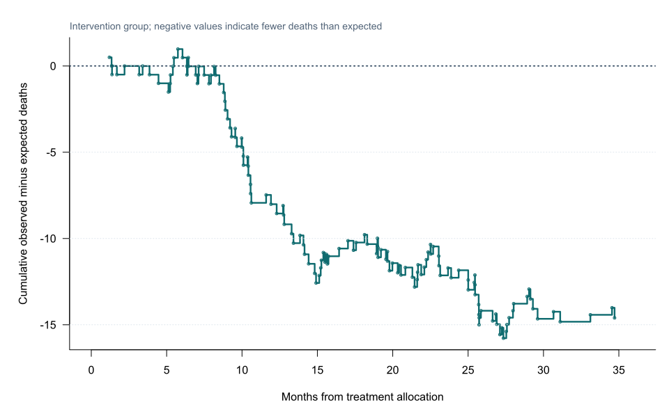
The cumulative score is descriptive. The formal test uses the final score and its variance.

Crossing survival curves

When curves cross, positive and negative event contributions can cancel.

A standard log-rank test may then have low power or give one global result that hides changing effects.

Possible responses include:

• prespecified weighted log-rank tests;
• time-specific survival differences;
• restricted mean survival time;
• time-varying Cox effects;
• milestone survival estimates.

Do not choose a weighted test after seeing which curve region gives the desired result.

Weighted log-rank tests

The Fleming–Harrington family applies weights based on the pooled survival estimate [3].

Different weights emphasise:

• early events;
• late events;
• middle follow-up.

The weight should reflect the expected clinical effect pattern and be prespecified.

Stratified log-rank tests

A stratified test compares groups within each stratum and combines the scores.

Use it when stratification was built into randomisation or when a prespecified nuisance factor should be controlled without estimating its effect directly.

The resulting test is still not a treatment-effect estimate.

Interpreting the output

Presenting the results

Suggested reporting

Report the test type, weighting, stratification, chi-square statistic, degrees of freedom and p-value.

Do not present the log-rank test as the sole result. A hazard ratio may be appropriate under proportional hazards, while restricted mean survival time can provide an alternative summary under non-proportional hazards [4].

Common mistakes

Knowledge check

What does the log-rank test compare at each event time?

Answer and reasoning

Observed and expected events based on the group-specific risk sets.

Is the log-rank test an effect estimate?

Answer and reasoning

No. It is a global hypothesis test.

Why can crossing curves reduce log-rank power?

Answer and reasoning

Event contributions in opposite directions can cancel over time.

When should a weighted log-rank test be used?

Answer and reasoning

When a particular early or delayed effect pattern is clinically expected and the weighting is prespecified.

What should accompany the log-rank result?

Answer and reasoning

Kaplan–Meier estimates, numbers at risk, confidence intervals and a clinically interpretable effect measure.

Key take-home messages

References

1. Mantel N. Evaluation of survival data and two new rank order statistics arising in its consideration. Cancer Chemother Rep. 1966;50(3):163–170.
2. Therneau TM. A package for survival analysis in R. R package survival version 3.8-9. 2026. https://CRAN.R-project.org/package=survival
3. Harrington DP, Fleming TR. A class of rank test procedures for censored survival data. Biometrika. 1982;69(3):553–566. https://doi.org/10.1093/biomet/69.3.553
4. Royston P, Parmar MKB. The use of restricted mean survival time to estimate the treatment effect in randomized clinical trials when the proportional hazards assumption is in doubt. Stat Med. 2011;30(19):2409–2421. https://doi.org/10.1002/sim.4274