Machine Learning versus Traditional Statistical Modelling

Overview

Machine learning and traditional statistical modelling overlap substantially.

Both can:

• fit regression functions;
• classify outcomes;
• regularise coefficients;
• estimate predictions;
• require validation.

The main distinction is often purpose and workflow rather than a strict algorithm boundary.

Why this matters

A complex algorithm can overfit, leak outcome information and fail in new settings.

A simple regression can also be badly specified.

Model choice should follow:

• intended use;
• sample size;
• outcome;
• data quality;
• required interpretability;
• validation plan.

When to use these approaches

Traditional modelling is often preferable when:

• effect estimation is primary;
• sample size is modest;
• predictor relationships are known;
• transparent coefficients are required.

Machine-learning workflows are useful when:

• prediction is primary;
• nonlinearities and interactions are complex;
• high-dimensional data exist;
• external validation is planned.

Research question and variables

The target is individual outcome probability.

Performance dimensions include:

• discrimination;
• calibration;
• Brier score;
• decision utility;
• fairness;
• transportability.

No one metric is sufficient.

Data structure

Prediction-development split

simulated data

Dataset	Purpose
Training	Fit and tune models
Validation	Tune hyperparameters
Test or external	Final performance assessment

Repeated cross-validation can combine training and validation, but final external assessment remains distinct.

Statistical assumptions

Traditional regression

Strengths include:

• interpretable coefficients;
• explicit uncertainty;
• flexible splines and interactions;
• causal estimands when designed appropriately.

Weaknesses arise from manual misspecification, overfitting and inappropriate significance-based selection.

Machine learning

Methods include:

• penalised regression;
• trees;
• random forests;
• gradient boosting;
• neural networks;
• support-vector machines.

Higher flexibility increases the need for regularisation and validation.

Worked example

Worked analysis in R

high_dimensional <- read.csv(
  "data/part-16-high-dimensional-data.csv"
)

set.seed(20260806)

train_index <- 1:600
test_index <- 601:800

x_names <- paste0(
  "x",
  1:30
)

traditional_fit <- glm(
  outcome ~ x1 + x2 +
    x3 + x4 + x5,
  data = high_dimensional[
    train_index,
  ],
  family = binomial
)

traditional_probability <- predict(
  traditional_fit,
  newdata = high_dimensional[
    test_index,
  ],
  type = "response"
)

x_train <- as.matrix(
  high_dimensional[
    train_index,
    x_names
  ]
)

x_test <- as.matrix(
  high_dimensional[
    test_index,
    x_names
  ]
)

lasso_fit <- glmnet::cv.glmnet(
  x_train,
  high_dimensional$outcome[
    train_index
  ],
  family = "binomial",
  alpha = 1
)

lasso_probability <- as.numeric(
  predict(
    lasso_fit,
    newx = x_test,
    s = "lambda.min",
    type = "response"
  )
)

Selected analysis output

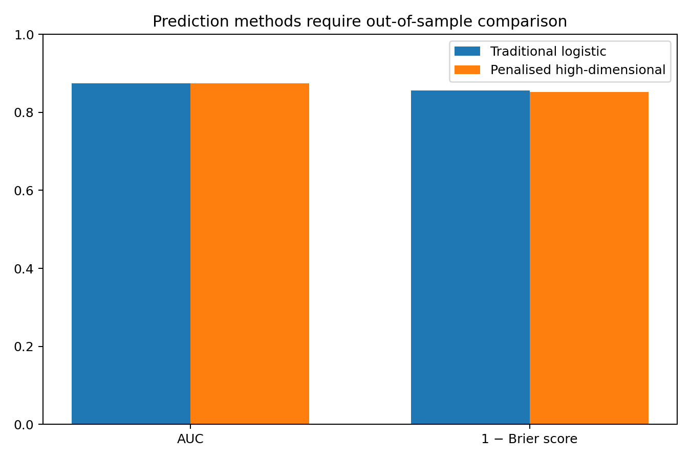
Traditional and lasso models have similar held-out AUCs and Brier scores.

The lasso retains a limited subset of non-zero coefficients.

Visualising model performance

Data leakage

Leakage occurs when information unavailable at prediction time enters model development.

Examples:

• using future laboratory values;
• imputing before data splitting;
• selecting predictors using the whole dataset;
• normalising using test data;
• repeated records crossing folds.

Leakage can produce impressive but invalid performance.

Interpretability

Coefficient visibility is not the same as clinical interpretability.

Interpretation tools include:

• partial dependence;
• accumulated local effects;
• SHAP values;
• variable importance.

These describe model behaviour, not causal effects.

Reporting and appraisal

TRIPOD+AI applies to regression and machine-learning prediction models [1].

PROBAST+AI addresses risk of bias and applicability [2].

Interpreting the output

Presenting the analysis

Suggested reporting

Report target population, outcome, prediction time, preprocessing, tuning, resampling, missing data, calibration, discrimination, utility, fairness and external validation [1], [2].

Statistical-learning and clinical-prediction texts provide broader foundations for algorithm complexity, validation and transportability [3], [4].

Common mistakes

Knowledge check

What distinguishes prediction from causal inference?

Answer and reasoning

Prediction estimates future outcomes; causal inference estimates intervention contrasts under causal assumptions.

What is leakage?

Answer and reasoning

Use of information unavailable at intended prediction time or improper use of validation data.

Why report calibration?

Answer and reasoning

A model can rank well while probabilities are systematically wrong.

Does SHAP show causal importance?

Answer and reasoning

No. It describes contribution within the fitted prediction model.

When should a simpler model be preferred?

Answer and reasoning

When performance and utility are similar and simplicity improves transparency or deployment.

Key take-home messages

References

1. Collins GS, Moons KGM, Dhiman P, Riley RD, Beam AL, Van Calster B, et al. TRIPOD+AI statement. BMJ. 2024;385:e078378. https://doi.org/10.1136/bmj-2023-078378
2. Moons KGM, Damen JAA, Kaul T, et al. PROBAST+AI. BMJ. 2025;388:e082505. https://doi.org/10.1136/bmj-2024-082505
3. Hastie T, Tibshirani R, Friedman J. The elements of statistical learning. 2nd ed. New York: Springer; 2009.
4. Steyerberg EW. Clinical prediction models. 2nd ed. Cham: Springer; 2019.