
Part 6 · Module 6
Repeated-Measures Analysis of Variance
Learn how to compare a numerical outcome across three or more repeated occasions using repeated-measures ANOVA, sphericity correction and reproducible R output.
Learning outcomes
After completing this lecture, you should be able to:
- Explain why repeated observations from one participant are correlated.
- State the time-effect null hypothesis in a one-factor repeated-measures ANOVA.
- Interpret the uncorrected and Greenhouse-Geisser-corrected F tests.
- Use multiplicity-adjusted paired comparisons to describe time-point differences.
- Recognise limitations of repeated-measures ANOVA with missing data and unequal timing.
- Use reproducible R code to fit and verify a balanced repeated-measures analysis.
Overview
Repeated-measures ANOVA compares a numerical outcome measured on the same participants at three or more occasions or conditions.
The method separates:
- stable between-participant differences;
- systematic differences across time or condition;
- residual within-participant variation.
Because measurements from one participant are correlated, ordinary one-way ANOVA is inappropriate.
This lecture presents the classical balanced one-factor repeated-measures ANOVA. Modern longitudinal studies often use linear mixed-effects models or generalised estimating equations because they handle incomplete data, unequal timing and flexible covariance structures more naturally [4], [5].
Why this matters
If 24 participants are measured at three visits, the dataset contains 72 rows but only 24 independent participants.
Treating all 72 observations as independent usually understates uncertainty.
Running three paired tests also fragments the research question and multiplies testing. Repeated-measures ANOVA provides one overall time test, followed by adjusted comparisons if required.
When to use this method
Use one-factor repeated-measures ANOVA when:
- one numerical outcome is measured at three or more occasions or conditions;
- the same independent participants contribute at every level;
- the design is balanced and complete or nearly so;
- the mean time or condition profile is the target;
- and covariance assumptions are sufficiently reasonable.
Prefer a mixed-effects model when:
- visits are missing;
- timing varies;
- participants have different numbers of observations;
- time is continuous;
- covariate-dependent trajectories are required;
- or a flexible covariance structure is needed.
Research question and variables
The outcome is systolic blood pressure.
The within-participant factor is time with three levels:
- baseline;
- month 3;
- month 6.
The estimand is the set of population mean differences across occasions.
For a study with treatment groups and time, a one-factor repeated-measures ANOVA is not enough. The primary treatment question usually concerns a group-by-time interaction or a prespecified time-specific contrast.
Data structure
Long repeated-measures structure
simulated data| participant_id | time | sbp_mmHg |
|---|---|---|
| P001 | Baseline | 153 |
| P001 | Month 3 | 148 |
| P001 | Month 6 | 153 |
| P002 | Baseline | 166 |
| P002 | Month 3 | 155 |
| P002 | Month 6 | 160 |
Note: The complete dataset contains 72 rows from 24 participants.
Participant identifier and time must uniquely identify each record.
Statistical assumptions
Sphericity
Sphericity requires equal variances of all pairwise difference scores among the repeated levels.
With exactly two levels, sphericity is automatic. With three or more, violation can make the uncorrected F test too liberal.
The Greenhouse–Geisser correction multiplies numerator and denominator degrees of freedom by an estimated epsilon between and 1 [1].
The F value remains unchanged, but the corrected p-value is larger.
How the method works
The repeated-measures ANOVA partitions variation into:
- time;
- participants;
- time-by-participant residual.
For the Greenhouse–Geisser correction:
Worked example
Reproducible R analysis
Base R can represent the participant and participant-by-time error strata using aov() with an Error() term [3].
wide <- data.frame(
  participant_id = factor(sprintf("P%03d", 1:24)),
  Baseline = c(
    153,166,154,160,157,157,136,162,156,137,143,146,
    169,165,149,144,140,140,143,144,155,148,139,155
  ),
  `Month 3` = c(
    148,155,146,159,152,151,127,150,149,136,141,146,
    174,162,147,137,136,137,134,142,147,143,131,151
  ),
  `Month 6` = c(
    153,160,145,139,149,141,137,150,139,122,135,124,
    158,157,143,132,124,136,136,130,146,137,133,139
  ),
  check.names = FALSE
)

long <- reshape(
  wide,
  varying = c("Baseline", "Month 3", "Month 6"),
  v.names = "sbp_mmHg",
  timevar = "time",
  times = c("Baseline", "Month 3", "Month 6"),
  direction = "long"
)

long$time <- factor(
  long$time,
  levels = c("Baseline", "Month 3", "Month 6")
)
long <- long[order(long$participant_id, long$time), ]

# Base R represents participant and participant-by-time error strata [3]
fit <- aov(
  sbp_mmHg ~ time + Error(participant_id / time),
  data = long
)

summary(fit)
R ANOVA output
Error: participant_id
          Df Sum Sq Mean Sq F value Pr(>F)
Residuals 23

Error: participant_id:time
          Df Sum Sq Mean Sq F value   Pr(>F)
time       2 1336.0   668.0   34.84 6.14e-10
Residuals 46  882.0    19.2
Greenhouse–Geisser epsilon in base R
S <- cov(wide[c("Baseline", "Month 3", "Month 6")])
k <- ncol(S)
Cmat <- diag(k) - matrix(1 / k, k, k)
S_centered <- Cmat %*% S %*% Cmat

epsilon_gg <- sum(diag(S_centered))^2 /
  ((k - 1) * sum(diag(S_centered %*% S_centered)))

F_time <- 34.8408
df1 <- 2
df2 <- 46

p_gg <- pf(
  F_time,
  df1 = epsilon_gg * df1,
  df2 = epsilon_gg * df2,
  lower.tail = FALSE
)

data.frame(
  epsilon_GG = epsilon_gg,
  corrected_df1 = epsilon_gg * df1,
  corrected_df2 = epsilon_gg * df2,
  F = F_time,
  p_value_GG = p_gg
)
Corrected output
 epsilon_GG corrected_df1 corrected_df2       F   p_value_GG
      0.631         1.262        29.017 34.8408 4.77e-07
Pairwise comparisons
p1 <- t.test(wide[["Month 3"]], wide$Baseline, paired = TRUE)
p2 <- t.test(wide[["Month 6"]], wide$Baseline, paired = TRUE)
p3 <- t.test(wide[["Month 6"]], wide[["Month 3"]], paired = TRUE)

raw_p <- c(p1$p.value, p2$p.value, p3$p.value)
holm_p <- p.adjust(raw_p, method = "holm")

pairwise_result <- data.frame(
  contrast = c(
    "Month 3 - Baseline",
    "Month 6 - Baseline",
    "Month 6 - Month 3"
  ),
  mean_difference = c(
    mean(wide[["Month 3"]] - wide$Baseline),
    mean(wide[["Month 6"]] - wide$Baseline),
    mean(wide[["Month 6"]] - wide[["Month 3"]])
  ),
  ci_lower = c(p1$conf.int[1], p2$conf.int[1], p3$conf.int[1]),
  ci_upper = c(p1$conf.int[2], p2$conf.int[2], p3$conf.int[2]),
  holm_p = holm_p
)

pairwise_result
Interpreting the output
Presenting the results
| Time | Mean (SD), mmHg |
|---|---|
| Baseline | 150.8 (9.7) |
| Month 3 | 145.9 (10.5) |
| Month 6 | 140.2 (10.6) |
Greenhouse–Geisser-corrected time effect: , , .
Visualising the results
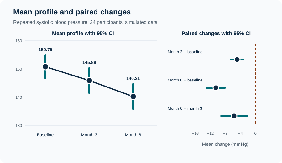
Suggested reporting
Why mixed-effects models are often preferable MMed extension
Classical repeated-measures ANOVA generally requires complete balanced data and a restrictive covariance assumption.
A linear mixed-effects model can:
- include participants with incomplete visits under stated missing-data assumptions;
- model unequal visit timing;
- include random effects;
- compare covariance structures;
- and estimate treatment-by-time contrasts.
The model should be chosen according to the estimand and study design rather than software convenience.
Common mistakes
Knowledge check
Why are 72 rows not 72 independent observations?
Answer and reasoning
They arise from 24 participants, each measured three times. Measurements within a participant are correlated.
What does sphericity concern?
Answer and reasoning
It concerns equality of variances of all pairwise difference scores among repeated levels.
What does the Greenhouse–Geisser correction change?
Answer and reasoning
It reduces the numerator and denominator degrees of freedom by epsilon, producing a more conservative p-value when sphericity is doubtful. The F value remains unchanged.
Why are pairwise visit comparisons adjusted?
Answer and reasoning
Three comparisons form a family. Holm adjustment limits family-wise type I error while identifying where differences occur.
When should a mixed model replace repeated-measures ANOVA?
Answer and reasoning
Common reasons include incomplete visits, unequal timing, flexible covariance needs, treatment-by-time modelling or participant-specific random effects.
Key take-home messages
References
- Greenhouse SW, Geisser S. On methods in the analysis of profile data. Psychometrika. 1959;24:95–112. https://doi.org/10.1007/BF02289823
- Geisser S, Greenhouse SW. An extension of Box’s results on the use of the F distribution in multivariate analysis. Ann Math Stat. 1958;29(3):885–891. https://doi.org/10.1214/aoms/1177706545
- R Core Team. Fit an analysis of variance model. R documentation, package stats version 4.6.1. Vienna: R Foundation for Statistical Computing; 2026. https://search.r-project.org/R/refmans/stats/html/aov.html
- Gueorguieva R, Krystal JH. Move over ANOVA: progress in analyzing repeated-measures data and its reflection in papers published in the Archives of General Psychiatry. Arch Gen Psychiatry. 2004;61(3):310–317. https://doi.org/10.1001/archpsyc.61.3.310
- Twisk JWR. Applied longitudinal data analysis for epidemiology. 2nd ed. Cambridge: Cambridge University Press; 2013. https://doi.org/10.1017/CBO9781139342834
These notes support learning and research planning and do not replace statistical consultation for a specific study.