Likelihood Ratios and Diagnostic Odds Ratio

Overview

Likelihood ratios combine sensitivity and specificity into factors that update diagnostic odds.

The positive likelihood ratio, $LR+$, describes how much more likely a positive result is among participants with the target condition than among those without it.

The negative likelihood ratio, $LR-$, describes how likely a negative result is among participants with the target condition relative to those without it.

Likelihood ratios connect diagnostic accuracy to Bayes’ theorem and can be applied across a range of pre-test probabilities [1].

The diagnostic odds ratio, DOR, combines $LR+$ and $LR-$ into one overall separation measure.

Why this matters

Sensitivity and specificity describe conditional classification, but clinicians often need to answer:

How should this result change the probability of disease?

Likelihood ratios provide that bridge.

However:

• an $LR+$ of 3.4 may be useful at one pre-test probability and insufficient at another;
• an $LR-$ of 0.21 reduces probability substantially but may not rule out a dangerous disease;
• a high DOR can arise from different sensitivity–specificity trade-offs.

Likelihood ratios and DOR should therefore be reported with clinical context and confidence intervals.

When to use these measures

Use likelihood ratios when:

• a test result must update a pre-test probability;
• the binary threshold and target condition are defined;
• sensitivity and specificity are applicable to the clinical setting;
• pre-test probability is estimated reasonably.

Likelihood ratios can also be defined for multiple result categories or intervals rather than only positive and negative results.

Research question and variables

For Test A:

$$LR+ = 0.842/0.250 = 3.37$$ $$LR- = 0.158/0.750 = 0.21$$

Data structure

Likelihood-ratio components

simulated data

Measure	Numerator	Denominator
$LR+$	Positive-result probability among diseased	Positive-result probability among non-diseased
$LR-$	Negative-result probability among diseased	Negative-result probability among non-diseased

Likelihood ratios use disease-specific probabilities rather than predictive-value denominators.

Statistical assumptions

Updating probability

Pre-test probability $p$ becomes pre-test odds:

At 30% pre-test probability:

$$\text{Pre-test odds} = 0.30/0.70 = 0.429$$

After a positive result:

$$0.429\times3.37 = 1.443$$ $$\text{Post-test probability} = 1.443/(1+1.443) = 59.1\%$$

After a negative result:

$$0.429\times0.21 = 0.090$$ $$\text{Post-test probability} = 0.090/(1+0.090) = 8.3\%$$

These equal the PPV and residual disease probability derived from the study table.

Worked example

Worked analysis in R

make_diagnostic_data <- function(n = 400) {
  id <- seq_len(n)
  age <- 20 + ((7 * id) %% 61)
  male <- as.integer(id %% 2 == 0)

  disease <- as.integer(
    ((id * 37) %% 100) < 30
  )

  score_a <-
    47 +
    11 * disease +
    0.08 * (age - 50) +
    7.5 * sin(id * 1.13) +
    3.5 * cos(id * 0.37)

  score_b <-
    48 +
    9 * disease +
    0.05 * (age - 50) +
    7.2 * sin(id * 1.13 + 0.45) +
    4.0 * cos(id * 0.37 + 0.20)

  disease_rank <- (id * 43) %% 100
  nondisease_rank <- (id * 47) %% 100

  reference_positive <- ifelse(
    disease == 1,
    disease_rank < 88,
    nondisease_rank >= 95
  )

  data.frame(
    id = id,
    age = age,
    male = male,
    disease = disease,
    score_a = score_a,
    score_b = score_b,
    reference_positive = as.integer(
      reference_positive
    )
  )
}

diagnostic_data <- make_diagnostic_data()

cutoff_a <- 51.962318662698785
cutoff_b <- 55.26626112612387

diagnostic_data$test_a_positive <- as.integer(
  diagnostic_data$score_a >= cutoff_a
)

diagnostic_data$test_b_positive <- as.integer(
  diagnostic_data$score_b >= cutoff_b
)

diagnostic_table <- with(
  diagnostic_data,
  table(
    test_a_positive,
    disease
  )
)

tn <- diagnostic_table["0", "0"]
fn <- diagnostic_table["0", "1"]
fp <- diagnostic_table["1", "0"]
tp <- diagnostic_table["1", "1"]

sensitivity <- tp / (tp + fn)
specificity <- tn / (tn + fp)

lr_positive <- sensitivity /
  (1 - specificity)

lr_negative <- (1 - sensitivity) /
  specificity

se_log_lr_positive <- sqrt(
  1 / tp -
  1 / (tp + fn) +
  1 / fp -
  1 / (fp + tn)
)

se_log_lr_negative <- sqrt(
  1 / fn -
  1 / (tp + fn) +
  1 / tn -
  1 / (fp + tn)
)

lr_positive_ci <- exp(
  log(lr_positive) +
  c(-1, 1) *
  qnorm(0.975) *
  se_log_lr_positive
)

lr_negative_ci <- exp(
  log(lr_negative) +
  c(-1, 1) *
  qnorm(0.975) *
  se_log_lr_negative
)

diagnostic_odds_ratio <-
  tp * tn / (fp * fn)

se_log_dor <- sqrt(
  1 / tp +
  1 / fn +
  1 / fp +
  1 / tn
)

dor_ci <- exp(
  log(diagnostic_odds_ratio) +
  c(-1, 1) *
  qnorm(0.975) *
  se_log_dor
)

c(
  lr_positive = lr_positive,
  lr_positive_lower = lr_positive_ci[1],
  lr_positive_upper = lr_positive_ci[2],
  lr_negative = lr_negative,
  lr_negative_lower = lr_negative_ci[1],
  lr_negative_upper = lr_negative_ci[2],
  diagnostic_odds_ratio = diagnostic_odds_ratio,
  dor_lower = dor_ci[1],
  dor_upper = dor_ci[2]
)

Selected analysis output

LR+ = 3.37 (95% CI 2.71 to 4.18)
LR− = 0.211 (95% CI 0.139 to 0.321)
DOR = 15.95 (95% CI 9.11 to 27.91)

Visualising probability updating

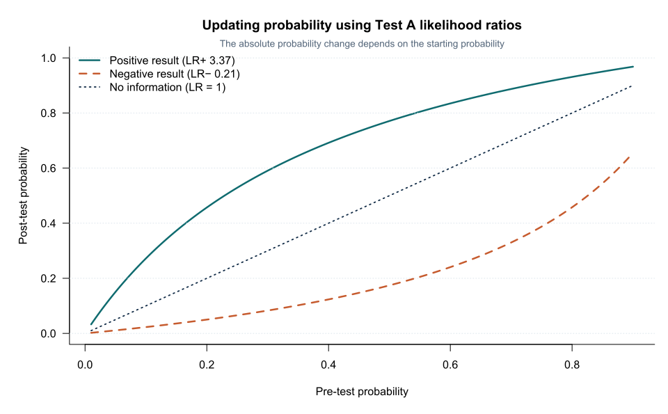
The diagonal represents no diagnostic information.

The positive-result curve lies above the diagonal because $LR+>1$.

The negative-result curve lies below because $LR-<1$.

Qualitative likelihood-ratio labels

Rules such as:

• $LR+>10$ strongly rules in;
• $LR-<0.1$ strongly rules out

can be useful approximations but should not replace probability calculation [2].

A test with $LR-=0.15$ may still leave an unacceptable post-test probability when the pre-test probability is high.

Diagnostic odds ratio

The DOR is frequently used in diagnostic meta-analysis because it provides one symmetric measure of discrimination [3].

Limitations include:

• loss of sensitivity–specificity trade-off;
• poor direct clinical interpretation;
• same DOR for different operating points;
• instability with zero cells;
• dependence on threshold and spectrum.

It should not be the only reported accuracy measure. Practical interpretation of likelihood ratios in diagnostic studies is also summarised by Deeks and Altman [4].

Sequential testing

When two tests are used sequentially:

$$\text{Post-test odds} = \text{Pre-test odds} \times LR_1 \times LR_2$$

only if the likelihood ratios are conditionally appropriate for the sequence.

Assuming independence between correlated tests can exaggerate probability updating.

The second-test likelihood ratio should ideally be estimated among patients reaching that stage of the pathway.

Interpreting the output

Presenting the results

Suggested reporting

Report likelihood ratios with confidence intervals and show probability updating for realistic pre-test values.

State whether results are binary, interval-specific or derived from sequential testing.

Common mistakes

Knowledge check

What quantity is multiplied by the likelihood ratio?

Answer and reasoning

Pre-test odds.

What does LR+ = 3.37 mean?

Answer and reasoning

A positive result is 3.37 times as likely among diseased participants as among non-diseased participants.

Does LR− = 0.21 rule out disease automatically?

Answer and reasoning

No. The residual probability depends on the pre-test probability and clinical action threshold.

What does the DOR conceal?

Answer and reasoning

The separate sensitivity–specificity trade-off and the clinical direction of errors.

Why can sequential LR multiplication fail?

Answer and reasoning

The tests may be conditionally dependent, and the second test may be used in a selected population.

Key take-home messages

References

1. Simel DL, Samsa GP, Matchar DB. Likelihood ratios with confidence: sample size estimation for diagnostic test studies. J Clin Epidemiol. 1991;44(8):763–770. https://doi.org/10.1016/0895-4356(91)90128-V
2. Jaeschke R, Guyatt GH, Sackett DL. Users’ guides to the medical literature. III. How to use an article about a diagnostic test. JAMA. 1994;271(9):703–707. https://doi.org/10.1001/jama.1994.03510330081039
3. Glas AS, Lijmer JG, Prins MH, Bonsel GJ, Bossuyt PMM. The diagnostic odds ratio: a single indicator of test performance. J Clin Epidemiol. 2003;56(11):1129–1135. https://doi.org/10.1016/S0895-4356(03)00177-X
4. Deeks JJ, Altman DG. Diagnostic tests 4: likelihood ratios. BMJ. 2004;329(7458):168–169. https://doi.org/10.1136/bmj.329.7458.168