
Part 12 · Module 2
Cohen's Kappa
Learn how Cohen's kappa measures chance-corrected agreement for two raters classifying the same participants into nominal categories.
Learning outcomes
After completing this lecture, you should be able to:
- Construct a paired nominal rating table for two raters.
- Calculate observed and expected agreement.
- Calculate and interpret Cohen's kappa and its confidence interval.
- Explain prevalence and marginal-distribution effects on kappa.
- Distinguish kappa from diagnostic accuracy and association.
- Use R code to report binary inter-rater agreement.
Overview
Cohen’s kappa measures agreement between two raters who classify the same participants into nominal categories [1].
It compares:
- observed agreement;
- agreement expected from the two raters’ marginal category proportions.
Kappa is often described as chance-corrected agreement.
It should be reported together with:
- the complete agreement table;
- observed agreement;
- category proportions;
- confidence interval;
- study context.
Why this matters
Observed agreement can be high when one category is very common.
Kappa adjusts for the agreement expected from the marginal distributions, but this creates well-known interpretation difficulties.
Two datasets can have the same observed agreement and different kappa values because category prevalence or rater bias differs.
Kappa is not:
- sensitivity;
- specificity;
- accuracy against a gold standard;
- correlation;
- proof that classifications are valid.
When to use Cohen’s kappa
Use Cohen’s kappa when:
- two raters or methods classify the same units;
- categories are nominal;
- every unit receives one classification from each rater;
- pairing is preserved;
- raters operate independently where feasible.
Use weighted kappa for ordinal categories when the severity of disagreement matters.
Use multi-rater extensions when more than two raters are involved.
Research question and variables
The agreement table is:
| Rater 2 absent | Rater 2 present | |
|---|---|---|
| Rater 1 absent | 81 | 7 |
| Rater 1 present | 5 | 67 |
Observed agreement is:
Data structure
Binary paired ratings
simulated data| Variable | Meaning |
|---|---|
id | Participant or image identifier |
binary_rater_1 | Rater 1 classification |
binary_rater_2 | Rater 2 classification |
One row belongs to one independently sampled item.
Statistical assumptions
How the method works
The expected agreement is calculated from the row and column marginals.
For the absent category:
For the present category:
Total expected agreement is:
Kappa is:
In the example:
Worked example
Worked analysis in R
rating_data <- read.csv(
  "data/part-12-rating-data.csv"
)

agreement_table <- with(
  rating_data,
  table(
    factor(
      binary_rater_1,
      levels = c(0, 1),
      labels = c("Absent", "Present")
    ),
    factor(
      binary_rater_2,
      levels = c(0, 1),
      labels = c("Absent", "Present")
    )
  )
)

observed_agreement <- sum(
  diag(agreement_table)
) / sum(agreement_table)

row_proportions <- rowSums(
  agreement_table
) / sum(agreement_table)

column_proportions <- colSums(
  agreement_table
) / sum(agreement_table)

expected_agreement <- sum(
  row_proportions *
  column_proportions
)

kappa <- (
  observed_agreement -
  expected_agreement
) / (
  1 - expected_agreement
)

agreement_table
c(
  observed_agreement = observed_agreement,
  expected_agreement = expected_agreement,
  kappa = kappa
)

irr::kappa2(
  rating_data[
    c(
      "binary_rater_1",
      "binary_rater_2"
    )
  ],
  weight = "unweighted"
)
Selected analysis output
                Rater 2
Rater 1        Absent Present
Absent             81       7
Present             5      67

Observed agreement = 0.925
Expected agreement = 0.504
Cohen's kappa = 0.849
Bootstrap 95% CI = 0.759 to 0.924
(The bootstrap confidence interval calculation is not shown here.)
Visualising categorical agreement
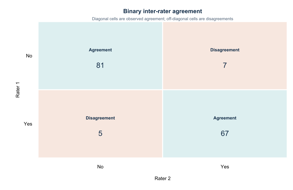
The off-diagonal pattern should be examined even when kappa is high.
Systematic directional disagreement may require retraining or clarification of category definitions.
Prevalence and bias effects
Kappa depends on the marginal category distributions.
When nearly every participant falls into one category:
- observed agreement can be high;
- expected agreement also becomes high;
- kappa can become modest.
This is often called the kappa prevalence paradox [2].
Rater bias occurs when raters use categories at different rates.
Report:
- category-specific counts;
- positive agreement;
- negative agreement;
- prevalence and bias indices where useful.
Interpretation labels
Common labels such as:
- slight;
- fair;
- moderate;
- substantial;
- almost perfect
are conventions rather than natural laws.
McHugh cautions that thresholds acceptable in one context may be unsafe in health research [3].
Clinical interpretation should consider:
- severity of disagreement;
- consequence of error;
- expected decision use;
- confidence interval;
- category prevalence.
Confidence intervals
A confidence interval quantifies sampling uncertainty.
Bootstrap intervals are useful when:
- analytic formulas are uncertain;
- tables are imbalanced;
- weighted or complex agreement statistics are used.
Resampling must preserve paired ratings by resampling units, not individual rater columns separately.
Kappa versus diagnostic accuracy
If one rater is a reference standard, sensitivity and specificity may be appropriate.
Kappa treats both raters symmetrically and does not designate one as truth.
High kappa does not establish that either rater is correct.
Alternatives
Alternatives include:
- Gwet’s agreement coefficients;
- prevalence-adjusted kappa;
- specific agreement;
- latent-class models.
These should be selected for a clear rationale rather than used only because ordinary kappa appears low. Gwet’s work provides one alternative framework when high marginal agreement destabilises ordinary kappa [4].
Interpreting the output
Presenting the results
Suggested reporting
Report the agreement table, observed agreement, kappa with CI, category definitions, rater training, blinding, participant spectrum and missing ratings.
Avoid reporting only an adjective such as “excellent agreement”.
Common mistakes
Knowledge check
What does observed agreement measure?
Answer and reasoning
The proportion of units classified identically by both raters.
What does kappa adjust for?
Answer and reasoning
Agreement expected from the two raters’ marginal category proportions.
Why can high observed agreement produce modest kappa?
Answer and reasoning
One category may dominate, making expected agreement high.
Does high kappa mean the classification is valid?
Answer and reasoning
No. Both raters can agree consistently on an incorrect classification.
Why examine off-diagonal cells?
Answer and reasoning
They show the direction and clinical type of disagreement that one summary coefficient conceals.
Key take-home messages
References
- Cohen J. A coefficient of agreement for nominal scales. Educ Psychol Meas. 1960;20(1):37–46. https://doi.org/10.1177/001316446002000104
- Feinstein AR, Cicchetti DV. High agreement but low kappa: I. The problems of two paradoxes. J Clin Epidemiol. 1990;43(6):543–549. https://doi.org/10.1016/0895-4356(90)90158-L
- McHugh ML. Interrater reliability: the kappa statistic. Biochem Med (Zagreb). 2012;22(3):276–282. https://doi.org/10.11613/BM.2012.031
- Gwet KL. Computing inter-rater reliability and its variance in the presence of high agreement. Br J Math Stat Psychol. 2008;61(1):29–48. https://doi.org/10.1348/000711006X126600
These notes support learning and research planning and do not replace statistical consultation for a specific study.