Interrupted Time-Series Analysis

Overview

Interrupted time-series, ITS, analysis evaluates a clearly timed intervention using repeated aggregate outcomes before and after implementation.

Segmented regression estimates:

• baseline level;
• pre-intervention trend;
• immediate level change;
• post-intervention slope change.

ITS is among the strongest quasi-experimental designs when randomisation is infeasible [1].

Why this matters

A simple before–after comparison cannot distinguish intervention effects from a pre-existing trend.

ITS can, but remains vulnerable to:

• simultaneous policies;
• coding changes;
• seasonality;
• autocorrelation;
• changing population composition.

When to use ITS

Use ITS when:

• intervention timing is clear;
• sufficient observations exist before and after;
• outcome measurement is stable;
• no randomised control is feasible;
• a comparable control series may be available.

Avoid using ITS with only a few time points.

Research question and variables

A segmented model is:

where:

• $\beta_1$ is pre-intervention slope;
• $\beta_2$ is immediate level change;
• $\beta_3$ is slope change.

Data structure

ITS variables

simulated data

Variable	Role
month	Sequential time
outcome	Monthly aggregate
post	0 before, 1 after intervention
time_after	Months since intervention

Statistical assumptions

Worked example

Worked analysis in R

its_data <- read.csv(
  "data/part-16-interrupted-time-series-data.csv"
)

its_fit <- lm(
  outcome ~ month +
    post +
    time_after,
  data = its_data
)

summary(its_fit)
confint(its_fit)

# Autocorrelation check
acf(
  residuals(its_fit)
)

# Newey–West sensitivity
lmtest::coeftest(
  its_fit,
  vcov. = sandwich::NeweyWest(
    its_fit,
    lag = 3,
    prewhite = FALSE
  )
)

Selected analysis output

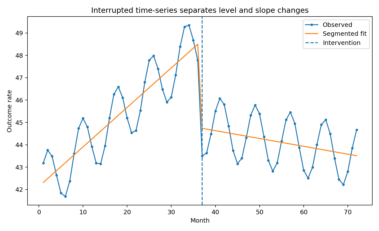
Pre-intervention slope ≈ 0.18 per month
Immediate level change ≈ -3.94
Slope change ≈ -0.21 per month
Post-intervention slope ≈ -0.04 per month

Visualising the interrupted series

Autocorrelation

Adjacent time points can be correlated.

Ignoring autocorrelation can produce incorrect SEs.

Options include:

• autoregressive errors;
• Newey–West SEs;
• generalised least squares;
• seasonal ARIMA errors.

The model should reflect the number and spacing of observations.

Controlled ITS

A control series helps address concurrent events.

A difference-in-differences ITS includes:

• group;
• time;
• intervention period;
• all relevant interactions.

The control should share external influences but not receive the intervention.

Interpreting the output

Presenting the analysis

Suggested reporting

Report intervention timing, number of points, outcome aggregation, model equation, autocorrelation, seasonality, co-interventions, control series and effect at meaningful post-intervention times [2].

Classical segmented-regression guidance and implementations for single- and multiple-group ITS designs are provided by Wagner and colleagues and Linden [3], [4].

Common mistakes

Knowledge check

What is the ITS counterfactual?

Answer and reasoning

The projected pre-intervention trend continued into the post-intervention period.

What does the level term estimate?

Answer and reasoning

Immediate change at the intervention time.

What does slope change estimate?

Answer and reasoning

Difference between post- and pre-intervention trends.

Why assess autocorrelation?

Answer and reasoning

Adjacent residuals may be dependent, affecting uncertainty.

What strengthens causal interpretation?

Answer and reasoning

A comparable control series and exclusion of concurrent changes.

Key take-home messages

References

1. Bernal JL, Cummins S, Gasparrini A. Interrupted time series regression for public health interventions. Int J Epidemiol. 2017;46(1):348–355. https://doi.org/10.1093/ije/dyw098
2. Jandoc R, Burden AM, Mamdani M, Lévesque LE, Cadarette SM. Interrupted time series analysis in drug utilisation research. J Clin Pharm Ther. 2015;40(4):365–372. https://doi.org/10.1111/jcpt.12268
3. Wagner AK, Soumerai SB, Zhang F, Ross-Degnan D. Segmented regression analysis of interrupted time series studies. J Clin Pharm Ther. 2002;27(4):299–309. https://doi.org/10.1046/j.1365-2710.2002.00430.x
4. Linden A. Conducting interrupted time-series analysis for single- and multiple-group comparisons. Stata J. 2015;15(2):480–500.