Mediation Analysis

Overview

Mediation analysis studies pathways through which an exposure affects an outcome.

A mediator occurs after exposure and contributes to the causal pathway.

The total effect may be decomposed into:

• direct effect;
• indirect effect through the mediator.

Causal mediation requires stronger assumptions than ordinary regression [1].

Why this matters

Adding a mediator to a regression model and observing that the treatment coefficient shrinks does not automatically establish mediation.

Bias can arise from:

• mediator–outcome confounding;
• treatment-induced confounding;
• measurement error;
• interaction;
• nonlinear models;
• temporal ambiguity.

When to use mediation analysis

Use mediation analysis when:

• a causal exposure is defined;
• mediator timing is clear;
• the target pathway is clinically meaningful;
• confounding assumptions are defensible;
• direct and indirect effects are prespecified.

Do not use mediation as an exploratory search among many post-treatment biomarkers without correction and validation.

Research question and variables

The linear path model is:

$$M=\alpha_0+aA+\boldsymbol\alpha^\top X+\varepsilon_M$$ $$Y=\beta_0+c'A+bM+\boldsymbol\beta^\top X+\varepsilon_Y$$

Without interaction and under linear assumptions:

Data structure

Mediation variables

simulated data

Variable	Role
treatment	Exposure
mediator	Post-treatment mediator
outcome	Clinical outcome
age, severity, comorbidity	Baseline covariates

Statistical assumptions

Natural and controlled effects

Natural direct and indirect effects compare mediator values under counterfactual treatment assignments.

They can be difficult to identify when treatment-induced confounders exist.

Controlled direct effects set the mediator to a fixed value.

The estimand should be stated rather than using “mediation effect” generically.

Worked example

Worked analysis in R

causal_data <- read.csv(
  "data/part-16-causal-data.csv"
)

mediator_fit <- lm(
  mediator ~ treatment +
    age +
    severity +
    comorbidity,
  data = causal_data
)

outcome_fit <- lm(
  outcome ~ treatment +
    mediator +
    age +
    severity +
    comorbidity,
  data = causal_data
)

a_path <- coef(
  mediator_fit
)["treatment"]

b_path <- coef(
  outcome_fit
)["mediator"]

direct_effect <- coef(
  outcome_fit
)["treatment"]

indirect_effect <- a_path *
  b_path

total_effect <- direct_effect +
  indirect_effect

c(
  direct = direct_effect,
  indirect = indirect_effect,
  total = total_effect
)

# mediation::mediate(...)
# sensitivity analysis:
# mediation::medsens(...)

Selected analysis output

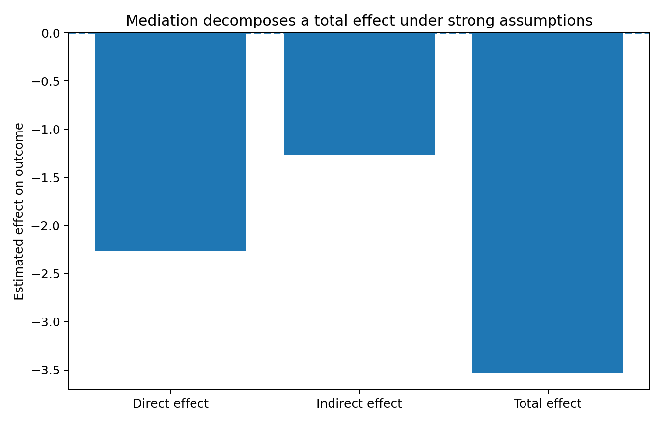
Direct effect ≈ -2.26
Indirect effect ≈ -1.27
Total effect ≈ -3.53

Visualising effect decomposition

Interaction and nonlinear outcomes

When treatment interacts with mediator, direct and indirect effects vary by treatment level.

For binary outcomes, decompositions on odds, risk or probability scales differ.

The simple $ab$ formula is generally inadequate.

Counterfactual or simulation-based methods are preferred.

Sensitivity analysis

Sensitivity analysis examines how strong unmeasured mediator–outcome confounding would need to be to change conclusions.

It does not prove the absence of confounding.

Interpreting the output

Presenting the analysis

Suggested reporting

Report temporal ordering, effect definitions, scale, interactions, confounders, missing data, bootstrap or simulation uncertainty and sensitivity analyses [2], [3].

Foundational work by Robins and Greenland clarifies identification of direct and indirect effects [4].

Common mistakes

Knowledge check

Why does treatment randomisation not solve all mediation confounding?

Answer and reasoning

The mediator is not randomised, so mediator–outcome confounding can remain.

What is the indirect effect in a simple linear model?

Answer and reasoning

The product of the treatment-to-mediator and mediator-to-outcome coefficients.

Why does scale matter?

Answer and reasoning

Direct and indirect effects differ on linear, risk, odds and hazard scales.

What can sensitivity analysis show?

Answer and reasoning

How conclusions change under specified unmeasured-confounding assumptions.

Does a smaller treatment coefficient after mediator adjustment prove mechanism?

Answer and reasoning

No.

Key take-home messages

References

1. VanderWeele TJ. Explanation in causal inference: methods for mediation and interaction. Oxford: Oxford University Press; 2015.
2. Imai K, Keele L, Tingley D. A general approach to causal mediation analysis. Psychol Methods. 2010;15(4):309–334. https://doi.org/10.1037/a0020761
3. Tingley D, Yamamoto T, Hirose K, Keele L, Imai K. mediation: R package for causal mediation analysis. J Stat Softw. 2014;59(5):1–38. https://doi.org/10.18637/jss.v059.i05
4. Robins JM, Greenland S. Identifiability and exchangeability for direct and indirect effects. Epidemiology. 1992;3(2):143–155.