Binary Logistic Regression

Overview

Binary logistic regression models a binary outcome using one or more predictors.

Examples include:

• controlled versus uncontrolled blood pressure;
• death versus survival;
• response versus no response;
• adverse event versus no adverse event.

The model uses the log odds, called the logit, because a straight linear model can otherwise predict probabilities below zero or above one.

Why this matters

Logistic coefficients are commonly exponentiated to odds ratios. Odds ratios are not risk ratios, especially when outcomes are common.

Predicted probabilities and absolute contrasts are often more clinically understandable than odds ratios alone.

When to use this method

Use binary logistic regression when:

• the outcome has two states;
• independent observations are available;
• adjusted conditional odds are the modelled scale;
• functional forms and sample information are adequate.

Use other models when repeated outcomes, clustering, time to event or direct risk ratios are the primary target.

Research question and variables

Data structure

Binary outcome coding

simulated data

Variable	Coding
Controlled outcome	1 = controlled, 0 = uncontrolled
Telemonitoring	1 = yes, 0 = usual care
Male	1 = male, 0 = female
Continuous predictors	Original clinical units

Statistical assumptions

How the method works

Maximum likelihood estimates coefficients that make the observed binary outcomes most probable under the model.

The intercept is usually not clinically interpretable when predictors equal zero outside plausible ranges.

Adjusted probabilities are obtained by applying:

$$p=\frac{e^\eta}{1+e^\eta}$$

to the linear predictor $\eta$.

Odds, probabilities and baseline risk

Odds are:

$$\text{odds}=\frac{p}{1-p}$$

A probability of 0.20 corresponds to odds 0.25, whereas a probability of 0.80 corresponds to odds 4.0. Because the conversion is nonlinear, one odds ratio can correspond to different probability differences at different baseline risks.

Clinical interpretation should therefore include predicted or standardised probabilities for relevant populations. Odds ratios remain useful model parameters but should not be translated directly into percentage changes in probability.

Continuous predictors and logit-linearity

A one-unit coefficient assumes a constant change in log odds across the predictor range. This does not imply a constant probability difference. Probability changes are greatest around intermediate risks and smaller near zero or one.

Assess functional form using clinical knowledge, plots and flexible terms such as restricted cubic splines. Categorising a continuous predictor is not a reliable solution to non-linearity.

Sparse data and separation

Sparse combinations of predictors and outcomes can produce very large coefficients and confidence intervals. Complete separation occurs when a predictor pattern perfectly divides events from non-events. The likelihood then has no finite maximum for the affected coefficient.

Possible responses include redesigning unsupported categories, collecting more information or using bias-reduced or penalised methods. Removing a clinically important predictor because the ordinary model fails is not a principled solution.

Model fit and calibration

A likelihood-ratio test compares nested logistic models. Measures such as AIC summarise relative fit, but neither establishes good probability calibration.

Calibration can be assessed by comparing predicted and observed risks over the prediction range. The Hosmer–Lemeshow test is sensitive to arbitrary grouping and sample size and should not be used as the sole model check.

Adjusted probabilities and marginal effects

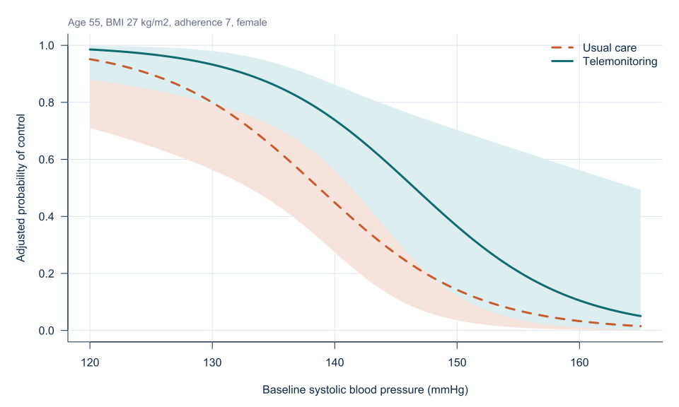
The coefficient describes a conditional odds ratio. To provide an adjusted absolute effect, predict each participant under both exposure values and average the resulting probabilities. This standardisation estimates a population-average risk contrast under the model.

A prediction for one reference profile can illustrate the model but should not be mistaken for the average treatment effect in the sample.

Classification thresholds

Converting probabilities into positive or negative classifications requires a threshold tied to clinical consequences. A threshold of 0.5 is not automatically optimal.

Sensitivity, specificity and accuracy change with the threshold and outcome prevalence. Model development should prioritise probability quality before classification performance.

Reporting

A reproducible logistic model requires the intercept, every coefficient, coding, transformations and interactions. A table of odds ratios alone is insufficient to reconstruct predicted probabilities.

Worked example

Reproducible R analysis

make_hypertension_data <- function(n = 180) {
  set.seed(4583)
  i <- seq_len(n)

  data <- data.frame(
    participant_id = sprintf("H%03d", i),
    age = round(runif(n, 30, 80)),
    male = rbinom(n, 1, 0.5),
    bmi = pmin(pmax(round(rnorm(n, 27, 3.5), 1), 18), 40),
    physical_activity = round(runif(n, 2, 7), 1),
    telemonitoring = rbinom(n, 1, 0.5)
  )

  data$adherence <- 4 + runif(n, 0, 5) -
    0.015 * (data$age - 55) + 0.4 * data$telemonitoring
  data$baseline_sbp <- 92 + 0.52 * data$age + 0.85 * data$bmi +
    2.8 * data$male - 1.3 * data$physical_activity + rnorm(n, 0, 4)
  data$followup_sbp <- 58 + 0.47 * data$baseline_sbp +
    0.10 * data$age + 0.52 * data$bmi - 2.0 * data$adherence +
    2.0 * data$male - 4.5 * data$telemonitoring -
    0.55 * data$telemonitoring * (data$bmi - 27) +
    0.006 * (data$age - 55)^2 + rnorm(n, 0, 5)

  data
}

hypertension <- make_hypertension_data()

hypertension$controlled <- as.integer(
  hypertension$followup_sbp < 130
)

fit <- glm(
  controlled ~ telemonitoring + baseline_sbp +
    age + bmi + adherence + male,
  data = hypertension,
  family = binomial(link = "logit")
)

summary(fit)

odds_ratios <- exp(coef(fit))
or_intervals <- exp(confint.default(fit))

reference_profiles <- data.frame(
  telemonitoring = c(0, 1),
  baseline_sbp = 140,
  age = 55,
  bmi = 27,
  adherence = 7,
  male = 0
)

predict(
  fit,
  newdata = reference_profiles,
  type = "response"
)

Cleaned R output

Predictor             Adjusted OR   95% CI
Telemonitoring           3.47       1.46 to 8.22
Baseline SBP             0.853      0.765 to 0.951
Age                      0.972      0.920 to 1.027
BMI                      0.909      0.787 to 1.051
Adherence                2.04       1.43 to 2.90
Male versus female       0.378      0.156 to 0.912

Base R fits logistic models using glm(..., family = binomial()) [1]. Model assessment should address fit, functional form, influence and separation [2], while regression specification and validation follow the intended estimand or prediction purpose [3].

Interpreting the output

Presenting the results

Present adjusted odds ratios with reference categories and supplement them with predicted probabilities for meaningful profiles.

Visualising predicted probabilities

Suggested reporting

Separation and penalisation MMed extension

When a predictor perfectly or almost perfectly classifies the outcome, maximum-likelihood coefficients can diverge. Penalised or bias-reduced logistic regression may be required rather than simply deleting the predictor or category.

Common mistakes

Knowledge check

What scale is linear in logistic regression?

Answer and reasoning

The log odds, not the probability itself.

Does OR = 3.47 mean probability is 3.47 times higher?

Answer and reasoning

No. The probability contrast depends on the starting risk and other predictor values.

What does an adherence OR of 3.07 mean?

Answer and reasoning

Each one-unit higher adherence score is associated with 3.07 times the adjusted odds of control, conditional on the model.

Why inspect logit-linearity?

Answer and reasoning

A continuous coefficient assumes a constant change in log odds per unit. Curvature makes that coefficient misleading.

What is separation?

Answer and reasoning

It occurs when predictor patterns perfectly or nearly perfectly determine outcome status, causing unstable maximum-likelihood estimates.

Key take-home messages

References

1. R Core Team. Fitting generalized linear models. R documentation, package stats version 4.6.1. Vienna: R Foundation for Statistical Computing; 2026. https://stat.ethz.ch/R-manual/R-devel/library/stats/html/glm.html
2. Hosmer DW, Lemeshow S, Sturdivant RX. Applied logistic regression. 3rd ed. Hoboken (NJ): Wiley; 2013. https://doi.org/10.1002/9781118548387
3. Harrell FE Jr. Regression modeling strategies. 2nd ed. Cham: Springer; 2015. https://doi.org/10.1007/978-3-319-19425-7