Competing-Risk Analysis

Overview

A competing event prevents the event of interest from occurring or changes its interpretation.

Examples include:

• death before disease recurrence;
• death before hospital discharge;
• transplantation before treatment failure;
• recovery before a particular complication;
• one cause of death when another cause occurs first.

For recurrence, death without recurrence is not ordinary loss to follow-up. The participant can no longer experience a first recurrence after death.

The probability of recurrence therefore depends on both:

• recurrence hazard;
• competing-death hazard.

Why this matters

If competing deaths are censored and one minus Kaplan–Meier is used as recurrence incidence, the method treats those deaths as though recurrence could still occur later.

This generally overestimates the real-world probability of recurrence [1].

The appropriate descriptive estimator is the cumulative incidence function, commonly estimated using the Aalen–Johansen approach.

Regression requires a clear choice between:

• cause-specific hazard;
• subdistribution hazard;
• direct risk or restricted-time estimands.

When to use this method

Use competing-risk analysis when one event prevents observation of the event of interest.

The competing event should be clinically defined before analysis.

Do not label ordinary loss to follow-up as a competing event.

Research question and variables

The event-of-interest estimand is:

$$F_1(t) = P(T\le t,\ J=1)$$

where:

• $T$ is time to the first event;
• $J=1$ denotes recurrence.

The competing-event cumulative incidence is:

$$F_2(t) = P(T\le t,\ J=2)$$

where $J=2$ denotes death without recurrence.

The event-free probability is:

$$S(t) = P(T>t)$$

For a complete competing-risk system:

$$S(t)+F_1(t)+F_2(t)=1$$

Data structure

Competing-risk status coding

simulated data

Status code	Meaning
0	Censored without recurrence or competing death
1	Recurrence
2	Death without previous recurrence

A factor-coded event status is useful for multi-state survival objects.

Statistical assumptions

How cumulative incidence works

At time $t_j$:

• $\widehat S(t_j-)$ is the estimated probability of being free of every event immediately before $t_j$;
• $d_{1j}$ is recurrence count;
• $n_j$ is the risk set.

The cumulative-incidence increment is:

The event-free survival falls after every event type, not only recurrence.

This is why competing deaths reduce later recurrence probability.

Worked example

Worked analysis in R

The survival package supports Aalen–Johansen multi-state curves through factor-coded Surv() outcomes and provides finegray() for Fine–Gray data expansion [2], [3].

make_survival_data <- function(n = 240) {
  id <- seq_len(n)
  group_numeric <- as.integer(id %% 2 == 0)
  age <- 35 + ((7 * id) %% 41)
  stage3 <- as.integer(id %% 3 == 0)

  deterministic_uniform <- function(multiplier) {
    (((id * multiplier) %% 997) + 0.5) / 998
  }

  u_recurrence <- deterministic_uniform(37)
  u_nonrecurrence_death <- deterministic_uniform(73)
  u_postrecurrence_death <- deterministic_uniform(109)
  u_dropout <- deterministic_uniform(149)
  u_dropout_time <- deterministic_uniform(181)

  recurrence_rate <-
    0.035 *
    exp(
      log(0.55) * group_numeric +
      0.025 * (age - 55) +
      0.55 * stage3
    )

  nonrecurrence_death_rate <-
    0.010 *
    exp(
      log(0.85) * group_numeric +
      0.030 * (age - 55) +
      0.40 * stage3
    )

  postrecurrence_death_rate <-
    0.060 *
    exp(
      log(0.85) * group_numeric +
      0.020 * (age - 55) +
      0.25 * stage3
    )

  recurrence_time <-
    -log(u_recurrence) / recurrence_rate

  nonrecurrence_death_time <-
    -log(u_nonrecurrence_death) /
    nonrecurrence_death_rate

  postrecurrence_death_delay <-
    -log(u_postrecurrence_death) /
    postrecurrence_death_rate

  overall_death_time <- pmin(
    nonrecurrence_death_time,
    recurrence_time +
      postrecurrence_death_delay
  )

  dropout_time <- ifelse(
    u_dropout < 0.22,
    12 + 24 * u_dropout_time,
    Inf
  )

  censor_time <- pmin(
    36,
    dropout_time
  )

  overall_time <- pmin(
    overall_death_time,
    censor_time
  )

  overall_event <- as.integer(
    overall_death_time <= censor_time
  )

  competing_time <- pmin(
    recurrence_time,
    nonrecurrence_death_time,
    censor_time
  )

  competing_status <- ifelse(
    recurrence_time <=
      nonrecurrence_death_time &
      recurrence_time <= censor_time,
    1L,
    ifelse(
      nonrecurrence_death_time <
        recurrence_time &
        nonrecurrence_death_time <=
          censor_time,
      2L,
      0L
    )
  )

  data.frame(
    id = id,
    group_numeric = group_numeric,
    group = factor(
      group_numeric,
      levels = c(0, 1),
      labels = c(
        "Usual care",
        "Intervention"
      )
    ),
    age = age,
    stage3 = stage3,
    stage = factor(
      stage3,
      levels = c(0, 1),
      labels = c("Stage II", "Stage III")
    ),
    overall_time = overall_time,
    overall_event = overall_event,
    competing_time = competing_time,
    competing_status = competing_status
  )
}

survival_data <- make_survival_data()

library(survival)

survival_data$competing_event <- factor(
  survival_data$competing_status,
  levels = c(0, 1, 2),
  labels = c(
    "censor",
    "recurrence",
    "death_without_recurrence"
  )
)

cif_fit <- survfit(
  Surv(
    competing_time,
    competing_event
  ) ~ group,
  data = survival_data
)

summary(
  cif_fit,
  times = c(12, 24, 36),
  extend = TRUE
)

# Cause-specific Cox model for recurrence
survival_data$age10 <-
  (survival_data$age - 55) / 10

cause_specific_fit <- coxph(
  Surv(
    competing_time,
    competing_status == 1
  ) ~ group + age10 + stage,
  data = survival_data,
  ties = "efron"
)

summary(cause_specific_fit)

# Fine–Gray subdistribution-hazard model
finegray_data <- finegray(
  Surv(
    competing_time,
    competing_event
  ) ~ group + age10 + stage + id,
  data = survival_data,
  etype = "recurrence"
)

finegray_fit <- coxph(
  Surv(
    fgstart,
    fgstop,
    fgstatus
  ) ~ group + age10 + stage +
    cluster(id),
  data = finegray_data,
  weights = fgwt
)

summary(finegray_fit)

Selected cumulative-incidence output

Recurrence CIF
Group          12 months   24 months   36 months
Usual care       0.358       0.563       0.672
Intervention     0.242       0.391       0.439

Death-without-recurrence CIF
Usual care       0.117       0.168       0.168
Intervention     0.108       0.144       0.229

Selected cause-specific recurrence model

Predictor                    Cause-specific HR   95% CI          p-value
Intervention                        0.519         0.364 to 0.741  <0.001
Age per 10 years                    1.315         1.134 to 1.525  <0.001
Stage III versus stage II           1.506         1.048 to 2.164   0.027

The Fine–Gray model targets a different hazard and should not be treated as a sensitivity version of the cause-specific Cox model.

Visualising cumulative incidence

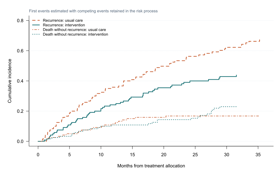
The sum of the two cumulative incidences and event-free probability remains one at each time.

Cause-specific hazard

The cause-specific recurrence hazard is the instantaneous recurrence rate among participants still alive and recurrence free.

For cause 1:

• participants experiencing recurrence leave the risk set as events;
• participants experiencing the competing event leave the risk set at that time;
• ordinary censoring also removes participants.

The cause-specific HR is useful for:

• aetiological questions;
• understanding event mechanisms;
• modelling all cause-specific hazards;
• deriving cumulative incidence from a complete set of hazards.

It does not directly state the effect on recurrence probability.

Fine–Gray subdistribution hazard

The Fine–Gray model links covariates to the subdistribution hazard associated with cumulative incidence [4].

Participants experiencing competing events remain in a weighted risk set.

The subdistribution HR is useful for modelling relative cumulative-incidence ordering, but it is not:

• a cause-specific HR;
• a risk ratio;
• an ordinary hazard among event-free participants.

Practical reporting recommendations emphasise stating the model and estimand explicitly [5].

Why one minus Kaplan–Meier is wrong

For recurrence, one minus a Kaplan–Meier curve that censors competing deaths estimates a hypothetical quantity in which recurrence could occur after those deaths.

The cumulative-incidence function estimates the observed-world probability of recurrence before or by time $t$ in the presence of competing death.

The two quantities answer different questions.

Choosing the regression model

Interpreting the output

Presenting the results

Suggested reporting

Report event definitions, counts for every cause, cumulative incidence at clinically relevant times, numbers at risk, regression estimand, hazard type, proportionality assessment and censoring assumptions.

Competing-risk guidance stresses that cause-specific and subdistribution models are complementary rather than interchangeable [1], [4], [5].

Common mistakes

Knowledge check

Why is death before recurrence a competing event?

Answer and reasoning

After death, a first recurrence cannot occur.

What does the cumulative incidence function estimate?

Answer and reasoning

The probability of experiencing a specific event type by time $t$ in the presence of competing events.

Why does one minus Kaplan–Meier overestimate recurrence probability?

Answer and reasoning

It censors competing deaths and behaves as though recurrence could occur after them.

What does a cause-specific HR compare?

Answer and reasoning

The instantaneous event-of-interest hazards among participants still free of every event.

Is a Fine–Gray HR a risk ratio?

Answer and reasoning

No. It is a proportional subdistribution-hazard parameter linked to cumulative incidence.

Key take-home messages

References

1. Andersen PK, Geskus RB, de Witte T, Putter H. Competing risks in epidemiology: possibilities and pitfalls. Int J Epidemiol. 2012;41(3):861–870. https://doi.org/10.1093/ije/dyr213
2. Aalen OO, Johansen S. An empirical transition matrix for non-homogeneous Markov chains based on censored observations. Scand J Stat. 1978;5(3):141–150.
3. Therneau TM. A package for survival analysis in R. R package survival version 3.8-9. 2026. https://CRAN.R-project.org/package=survival
4. Fine JP, Gray RJ. A proportional hazards model for the subdistribution of a competing risk. J Am Stat Assoc. 1999;94(446):496–509. https://doi.org/10.1080/01621459.1999.10474144
5. Austin PC, Lee DS, Fine JP. Introduction to the analysis of survival data in the presence of competing risks. Circulation. 2016;133(6):601–609. https://doi.org/10.1161/CIRCULATIONAHA.115.017719