Diagnostic Accuracy with Imperfect Reference Standards

Overview

A reference standard classifies the target condition against which the index test is evaluated.

In many clinical problems, no reference standard is perfectly sensitive and specific.

Examples include:

• culture for infections;
• histopathology with sampling error;
• expert consensus;
• composite clinical criteria;
• long-term follow-up;
• imaging interpretations;
• latent or evolving conditions.

Treating an imperfect reference as error free can bias every apparent accuracy measure.

The direction and magnitude depend on:

• reference sensitivity and specificity;
• disease prevalence;
• conditional dependence between tests;
• verification mechanism;
• participant spectrum.

Why this matters

An index test can be classified as “false positive” when it correctly detects disease missed by the reference standard.

It can be classified as “false negative” when the reference creates a false-positive disease label.

The apparent 2 × 2 table then compares two fallible measurements rather than one test against truth.

No-gold-standard analysis requires stronger modelling assumptions, not weaker reporting.

When this problem occurs

Consider imperfect-reference methods when:

• the accepted standard has known error;
• verification is unavailable for some participants;
• several tests measure the same latent condition;
• clinical follow-up is used as part of diagnosis;
• no single procedure is ethically or practically definitive.

The primary scientific question should still define the target condition precisely.

Research question and variables

Let:

• $D$ be the unobserved true target condition;
• $R$ be the observed reference classification;
• $T$ be the index-test classification.

The ordinary apparent analysis estimates:

$$P(T=1\mid R=1)$$

and:

$$P(T=0\mid R=0)$$

These equal true sensitivity and specificity only if $R=D$ without error or under special assumptions.

Data structure

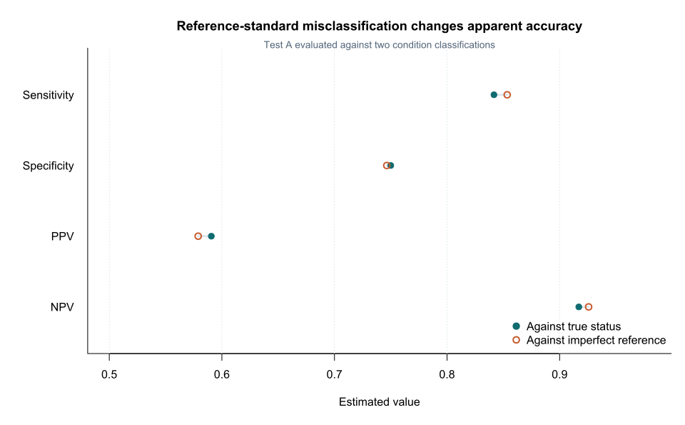
True and apparent accuracy in the simulation

simulated data

Measure	Against true condition	Against imperfect reference
Sensitivity	84.2%	85.3%
Specificity	75.0%	74.6%
PPV	59.1%	57.9%
NPV	91.7%	92.6%
Diagnostic odds ratio	15.95	17.15

Note: The apparent estimates are not uniformly closer to or farther from the truth.

The modest differences in this example should not imply imperfect references are harmless. Bias can be much larger under other errors and dependencies.

Statistical assumptions

Reference misclassification

Suppose reference sensitivity is less than 100%.

Some truly diseased participants appear in the reference-negative group.

If the index test identifies them, they are counted as apparent false positives, reducing apparent specificity.

Reference false positives can place truly non-diseased participants in the reference-positive group, altering apparent sensitivity.

Conditional dependence can reverse simple expectations.

Worked example

Worked analysis in R

make_diagnostic_data <- function(n = 400) {
  id <- seq_len(n)
  age <- 20 + ((7 * id) %% 61)
  male <- as.integer(id %% 2 == 0)

  disease <- as.integer(
    ((id * 37) %% 100) < 30
  )

  score_a <-
    47 +
    11 * disease +
    0.08 * (age - 50) +
    7.5 * sin(id * 1.13) +
    3.5 * cos(id * 0.37)

  score_b <-
    48 +
    9 * disease +
    0.05 * (age - 50) +
    7.2 * sin(id * 1.13 + 0.45) +
    4.0 * cos(id * 0.37 + 0.20)

  disease_rank <- (id * 43) %% 100
  nondisease_rank <- (id * 47) %% 100

  reference_positive <- ifelse(
    disease == 1,
    disease_rank < 88,
    nondisease_rank >= 95
  )

  data.frame(
    id = id,
    age = age,
    male = male,
    disease = disease,
    score_a = score_a,
    score_b = score_b,
    reference_positive = as.integer(
      reference_positive
    )
  )
}

diagnostic_data <- make_diagnostic_data()

cutoff_a <- 51.962318662698785
cutoff_b <- 55.26626112612387

diagnostic_data$test_a_positive <- as.integer(
  diagnostic_data$score_a >= cutoff_a
)

diagnostic_data$test_b_positive <- as.integer(
  diagnostic_data$score_b >= cutoff_b
)

accuracy_table <- function(
  test_positive,
  reference_positive
) {
  tab <- table(
    factor(
      test_positive,
      levels = c(1, 0)
    ),
    factor(
      reference_positive,
      levels = c(1, 0)
    )
  )

  tp <- tab["1", "1"]
  fp <- tab["1", "0"]
  fn <- tab["0", "1"]
  tn <- tab["0", "0"]

  data.frame(
    tp = tp,
    fn = fn,
    fp = fp,
    tn = tn,
    sensitivity = tp / (tp + fn),
    specificity = tn / (tn + fp),
    ppv = tp / (tp + fp),
    npv = tn / (tn + fn),
    dor = tp * tn / (fp * fn)
  )
}

true_accuracy <- accuracy_table(
  diagnostic_data$test_a_positive,
  diagnostic_data$disease
)

apparent_accuracy <- accuracy_table(
  diagnostic_data$test_a_positive,
  diagnostic_data$reference_positive
)

rbind(
  true_target_condition = true_accuracy,
  imperfect_reference = apparent_accuracy
)

Selected analysis output

Reference                 Sensitivity Specificity PPV   NPV   DOR
True target condition       0.842       0.750    0.591 0.917 15.95
Imperfect reference         0.853       0.746    0.579 0.926 17.15

Visualising apparent-reference bias

Composite reference standards

A composite reference combines several sources.

Rules include:

• disease if any component is positive;
• disease if all are positive;
• disease if a predefined combination is met;
• expert panel adjudication.

Advantages:

• may improve sensitivity;
• can integrate clinically relevant evidence.

Risks:

• components may include the index test;
• rules can be data driven;
• dependency is concealed;
• reproducibility is poor;
• incorporation bias occurs.

The rule should be prespecified and reproducible.

Discrepant analysis

Discrepant analysis applies additional testing mainly when the index and reference disagree.

This is generally biased because the resolution process depends on the index-test result.

It can make the index test appear more accurate by selectively overturning apparent errors.

Discrepant analysis should not be presented as an unbiased correction.

Differential verification

Different reference standards may be used according to the index-test result.

Example:

• biopsy after positive imaging;
• clinical follow-up after negative imaging.

This can create differential classification and verification bias.

A review of solutions for imperfect and missing reference standards emphasises that the method must match the verification mechanism [1]. Methods may require:

• inverse-probability weighting;
• multiple imputation;
• joint modelling;
• sensitivity analysis.

Latent-class models

Latent-class models treat true disease status as unobserved.

A basic model estimates:

• prevalence;
• sensitivities;
• specificities;
• dependence parameters.

Two tests in one population are generally not identifiable without strong assumptions.

The Hui–Walter framework uses at least two populations with different prevalences and at least two tests under conditional-independence assumptions [2].

Bayesian latent-class models can incorporate prior information but do not eliminate identifiability concerns.

Conditional dependence

Two tests can share biological or measurement mechanisms.

Examples:

• two antibody assays;
• two radiologists reading the same image;
• index test and composite reference using the same biomarker.

Assuming conditional independence when dependence exists can bias latent-class accuracy.

Dependence terms or sensitivity analyses may be required.

Sensitivity analysis

When reference accuracy is uncertain, vary plausible values.

For each assumed reference sensitivity and specificity, examine:

• corrected prevalence;
• corrected test accuracy;
• whether conclusions change;
• whether any corrected values become impossible.

The uncertainty range should come from external evidence or expert elicitation rather than arbitrary convenience. Classical correction and misclassification frameworks are reviewed by Walter and Irwig [3].

Interpreting the output

Presenting the results

Suggested reporting

Use STARD 2015 for diagnostic accuracy reporting [4]. For Bayesian latent-class models, STARD-BLCM specifies reporting of model structure, priors, dependence, identifiability, computation and sensitivity analyses [5].

Common mistakes

Knowledge check

Why can an index true positive be labelled false positive?

Answer and reasoning

The imperfect reference may miss the disease and classify that participant as reference negative.

What is incorporation bias?

Answer and reasoning

The index test contributes to the reference classification, creating artificial agreement.

Why is discrepant analysis biased?

Answer and reasoning

Additional reference testing is triggered by disagreement with the index test.

What is identifiability?

Answer and reasoning

Whether the observed data and assumptions contain enough information to estimate the model parameters uniquely.

Does Bayesian modelling solve absent information automatically?

Answer and reasoning

No. Priors and structural assumptions supply information and must be justified and tested.

Key take-home messages

References

1. Reitsma JB, Rutjes AWS, Khan KS, Coomarasamy A, Bossuyt PMM. A review of solutions for diagnostic accuracy studies with an imperfect or missing reference standard. J Clin Epidemiol. 2009;62(8):797–806. https://doi.org/10.1016/j.jclinepi.2009.02.005
2. Hui SL, Walter SD. Estimating the error rates of diagnostic tests. Biometrics. 1980;36(1):167–171. https://doi.org/10.2307/2530508
3. Walter SD, Irwig LM. Estimation of test error rates, disease prevalence and relative risk from misclassified data: a review. J Clin Epidemiol. 1988;41(9):923–937. https://doi.org/10.1016/0895-4356(88)90110-2
4. Bossuyt PM, Reitsma JB, Bruns DE, Gatsonis CA, Glasziou PP, Irwig L, et al. STARD 2015: an updated list of essential items for reporting diagnostic accuracy studies. BMJ. 2015;351:h5527. https://doi.org/10.1136/bmj.h5527
5. Kostoulas P, Nielsen SS, Branscum AJ, Johnson WO, Dendukuri N, Dhand NK, et al. STARD-BLCM: standards for the reporting of diagnostic accuracy studies that use Bayesian latent class models. Prev Vet Med. 2017;138:37–47. https://doi.org/10.1016/j.prevetmed.2017.01.006