Non-Linearity in Regression

Overview

Regression does not require predictors to be normally distributed. It requires their relationship with the modelled outcome scale to be represented adequately.

A continuous predictor may have:

• a linear relation;
• a threshold-like pattern;
• a plateau;
• a U-shaped relation;
• another smooth curve.

Forcing a straight line can bias estimates and conceal clinically important patterns.

Why this matters

Categorising a continuous predictor into normal and high values discards information and imposes an abrupt jump at the cut-off.

Flexible modelling usually preserves more information and allows the data to show gradual change, while still requiring control of overfitting [1].

When to use this method

Assess non-linearity when a continuous predictor is clinically important and the relation is not known to be linear.

Methods include:

• transformations;
• polynomial terms;
• restricted cubic splines;
• fractional polynomials;
• smoothers used with appropriate validation.

Research question and variables

Age is centred at 55 years:

$$A_c=A-55$$

The quadratic model is:

Data structure

Why centring helps

simulated data

Age	Centred age	Squared centred age
40	−15	225
55	0	0
70	15	225

Statistical assumptions

How the method works

A quadratic term allows one bend but can behave implausibly outside the observed range.

Restricted cubic splines use piecewise cubic functions joined smoothly and constrained to be linear in the tails [2].

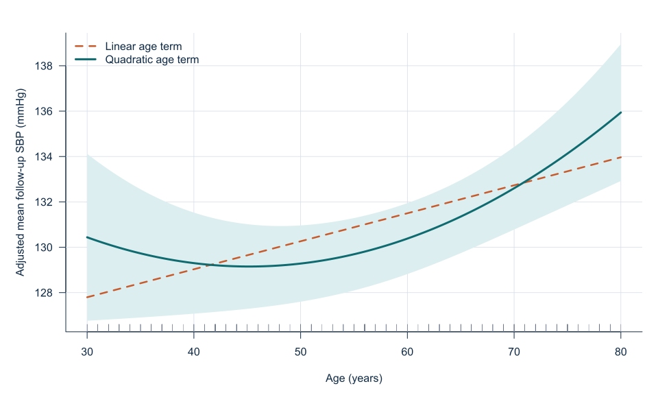
The curve should be reported through predicted values or contrasts rather than interpreting higher-order coefficients alone.

Recognising non-linearity

Non-linearity can be suspected from:

• a scatter plot or partial-residual plot;
• systematic curvature in residuals;
• implausible predictions at the ends of the range;
• clinical knowledge of thresholds, saturation or U-shaped effects.

A formal test can support a comparison, but failure to reject linearity does not prove that a straight line is adequate. The sample may contain too little information at the extremes.

Polynomial models

A quadratic model permits one U-shaped or inverted-U bend. The linear and squared terms should be retained together even if one coefficient is not individually significant.

Polynomial coefficients are difficult to interpret directly and can become unstable when the predictor is not centred. Higher-degree polynomials can oscillate and extrapolate dramatically, so they are rarely a good default for clinical modelling.

Restricted cubic splines

A restricted cubic spline divides the predictor range using knots and fits connected cubic pieces. The curve and its first two derivatives join smoothly. Linear restrictions in the tails reduce unstable extrapolation.

Spline interpretation should focus on:

• a graph of adjusted predictions;
• contrasts relative to a meaningful reference;
• an overall test of the predictor;
• an additional test of nonlinear components where relevant.

Individual spline-basis coefficients are not clinically meaningful.

Choosing knots and complexity

Knots are often placed at prespecified predictor quantiles. More knots permit greater flexibility but consume more parameters and can overfit sparse tails.

The choice should reflect sample size, anticipated biological complexity and the purpose of the model. Prediction models may use flexible terms with shrinkage, whereas a small explanatory study may need a parsimonious prespecified form.

Non-linearity in generalised models

The relevant scale changes with the model:

• linear regression: mean outcome;
• logistic regression: log odds;
• Poisson regression: log rate;
• Cox regression: log hazard.

A straight relation in probability is not the same as a straight relation in log odds. Plot predictions on the clinical scale even when estimation occurs on a transformed link scale.

Comparing models

Nested likelihood-ratio or partial F tests can compare a linear model with a richer nonlinear specification. Information criteria and cross-validated prediction error can also inform choice.

The selected form should not be determined by one test alone. Clinical plausibility, stability, uncertainty and visual agreement matter.

Reporting the curve

Provide the observed predictor distribution beneath or alongside the fitted curve so readers can identify sparse regions. Show confidence bands and avoid extending the graph beyond the data merely to make the line visually complete.

Worked example

Reproducible R analysis

make_hypertension_data <- function(n = 180) {
  set.seed(4583)
  i <- seq_len(n)

  data <- data.frame(
    participant_id = sprintf("H%03d", i),
    age = round(runif(n, 30, 80)),
    male = rbinom(n, 1, 0.5),
    bmi = pmin(pmax(round(rnorm(n, 27, 3.5), 1), 18), 40),
    physical_activity = round(runif(n, 2, 7), 1),
    telemonitoring = rbinom(n, 1, 0.5)
  )

  data$adherence <- 4 + runif(n, 0, 5) -
    0.015 * (data$age - 55) + 0.4 * data$telemonitoring
  data$baseline_sbp <- 92 + 0.52 * data$age + 0.85 * data$bmi +
    2.8 * data$male - 1.3 * data$physical_activity + rnorm(n, 0, 4)
  data$followup_sbp <- 58 + 0.47 * data$baseline_sbp +
    0.10 * data$age + 0.52 * data$bmi - 2.0 * data$adherence +
    2.0 * data$male - 4.5 * data$telemonitoring -
    0.55 * data$telemonitoring * (data$bmi - 27) +
    0.006 * (data$age - 55)^2 + rnorm(n, 0, 5)

  data
}

hypertension <- make_hypertension_data()

hypertension$age_c <- hypertension$age - 55

linear_age <- lm(
  followup_sbp ~ baseline_sbp + telemonitoring +
    bmi + adherence + male + age_c,
  data = hypertension
)

quadratic_age <- lm(
  followup_sbp ~ baseline_sbp + telemonitoring +
    bmi + adherence + male + age_c + I(age_c^2),
  data = hypertension
)

anova(linear_age, quadratic_age)
summary(quadratic_age)
confint(quadratic_age)

age_grid <- data.frame(
  baseline_sbp = mean(hypertension$baseline_sbp),
  telemonitoring = 0,
  bmi = mean(hypertension$bmi),
  adherence = mean(hypertension$adherence),
  male = 0,
  age_c = seq(-25, 25, by = 1)
)

age_grid$predicted <- predict(
  quadratic_age,
  newdata = age_grid
)

plot(
  age_grid$age_c + 55,
  age_grid$predicted,
  type = "l",
  xlab = "Age (years)",
  ylab = "Adjusted mean follow-up SBP (mmHg)"
)

Cleaned R output

Term             Estimate   95% CI              p-value
Centred age       0.110     0.007 to 0.213       0.036
Centred age²      0.00560   0.00143 to 0.00976   0.009

Nested-model F(1,172) = 7.02, p = 0.009

Interpreting the output

Presenting the results

Present the fitted curve and uncertainty across the observed predictor range rather than only higher-order coefficients.

Visualising non-linearity

Suggested reporting

Restricted cubic splines MMed extension

Base R provides natural cubic splines using splines::ns(). Knot number and placement should be prespecified or validated. The overall non-linear contribution can be assessed by comparing the spline model with its linear counterpart [2], [3].

Common mistakes

Knowledge check

Does linear regression require age to be normally distributed?

Answer and reasoning

No. The relevant issue is whether the conditional mean relation and residual assumptions are suitable.

Why centre age before squaring it?

Answer and reasoning

It improves interpretability and reduces unnecessary correlation between the linear and squared terms.

What does a significant quadratic term establish?

Answer and reasoning

It supports curvature under the fitted specification, not the universal truth of a quadratic relation.

Why avoid age categories?

Answer and reasoning

Categories discard ordering and within-category information and impose abrupt boundaries.

How should a non-linear result be reported?

Answer and reasoning

Use a graph and clinically relevant predicted contrasts with confidence intervals.

Key take-home messages

References

1. Royston P, Altman DG, Sauerbrei W. Dichotomizing continuous predictors in multiple regression: a bad idea. Stat Med. 2006;25(1):127–141. https://doi.org/10.1002/sim.2331
2. Harrell FE Jr. Regression modeling strategies. 2nd ed. Cham: Springer; 2015. https://doi.org/10.1007/978-3-319-19425-7
3. R Core Team. Regression splines. R documentation, package splines version 4.6.1. Vienna: R Foundation for Statistical Computing; 2026. https://stat.ethz.ch/R-manual/R-devel/library/splines/html/ns.html