Analysis of Repeated Trial Outcomes

Overview

Repeated trial outcomes contain several measurements from each participant.

The analysis should estimate a coherent longitudinal treatment effect rather than perform separate tests at every visit.

Common methods include:

• mixed models for repeated measures;
• random-effects models;
• generalised estimating equations;
• constrained longitudinal data analysis.

Why this matters

Separate visit tests:

• ignore within-participant correlation;
• create multiplicity;
• can produce inconsistent conclusions;
• fail to describe the treatment trajectory.

Repeated models can use incomplete outcome profiles under explicit assumptions.

When to use these methods

Use repeated-outcome methods when:

• the same endpoint is measured at several times;
• trajectory or time-specific treatment effects matter;
• participants have incomplete visit patterns;
• within-participant correlation must be modelled.

A final-visit ANCOVA remains appropriate when the final visit is the sole primary estimand and missing data are handled suitably.

Research question and variables

Possible estimands include:

• month-6 mean difference;
• average treatment effect over follow-up;
• difference in linear slopes;
• area under the mean trajectory;
• probability of response over time.

The simulated model uses:

• treatment group;
• categorical month;
• treatment-by-month interaction;
• participant random intercept.

Data structure

Long-format trial data

simulated data

Variable	Role
id	Participant cluster
group	Assigned treatment
month	Repeated visit
outcome	Numerical outcome
site	Trial site

Statistical assumptions

Mixed model for repeated measures

A common model is:

A categorical-time MMRM often models an unstructured or other residual covariance without a random intercept.

A random-intercept model provides a conditional trajectory.

GEE versus mixed models

GEE estimates population-average effects.

Mixed models estimate conditional effects and variance components.

For Gaussian identity-link outcomes, fixed mean contrasts are often numerically similar.

For binary outcomes, marginal and subject-specific effects differ.

Worked example

Worked analysis in R

trial_long <- read.csv(
  "data/part-13-repeated-trial-data.csv"
)

library(lme4)

mixed_fit <- lmer(
  outcome ~ group * month +
    factor(site) +
    (1 | id),
  data = trial_long,
  REML = TRUE
)

summary(mixed_fit)
confint(
  mixed_fit,
  parm = "beta_",
  method = "Wald"
)

observed_means <- aggregate(
  outcome ~ group_label + month,
  data = trial_long,
  FUN = function(x) {
    c(
      n = sum(!is.na(x)),
      mean = mean(x, na.rm = TRUE),
      sd = sd(x, na.rm = TRUE)
    )
  }
)

observed_means

Selected analysis output

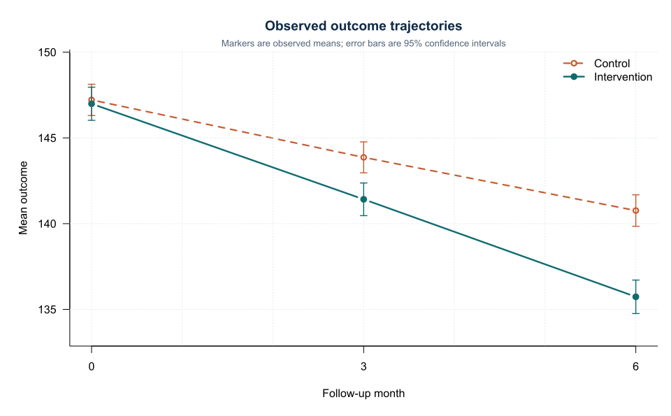
The treatment-by-month coefficient is approximately -0.75 units per month.

Observed group means are similar at baseline and progressively separated at months 3 and 6.

Exact mixed-model output can vary with the software package’s denominator-degrees-of-freedom and covariance conventions, so readers should confirm those settings when reproducing the analysis.

Visualising repeated trial outcomes

Baseline handling

Options include:

• baseline as a covariate with post-baseline outcomes;
• constrained longitudinal analysis including baseline as an outcome and constraining baseline group means equal;
• change-score modelling.

The choice should be prespecified and coherent with randomisation.

Missing repeated outcomes

Likelihood-based mixed models are commonly valid under missing at random conditional on included history and model.

Sensitivity analyses can include:

• delta-adjusted pattern-mixture models;
• reference-based imputation;
• tipping-point analyses;
• dropout-pattern models.

The strategy should align with the estimand.

Multiplicity

When one visit is primary, clearly label it.

When several visits are confirmatory, control type I error or use a global estimand.

Post hoc focus on the visit with the strongest result is selective reporting.

Interpreting the output

Presenting the results

Suggested reporting

Report visit counts, observed means, covariance or random-effects structure, estimation method, treatment-by-time test, time-specific contrasts, missing-data assumptions and sensitivity analyses.

Longitudinal trial modelling, MMRM practice, reference-based sensitivity analysis and estimand alignment are described in established guidance [1], [2], [3], [4].

Common mistakes

Knowledge check

What does treatment by time represent?

Answer and reasoning

How the treatment contrast changes across time on the model scale.

Why avoid separate tests at each visit?

Answer and reasoning

They ignore the coherent trajectory and create multiplicity.

What is the main difference between GEE and mixed models?

Answer and reasoning

GEE targets marginal population-average effects; mixed models include subject- or cluster-specific random effects.

Does MAR mean missingness is random without conditions?

Answer and reasoning

No. It is conditional on observed variables included in the analysis model.

What should be reported instead of only the interaction coefficient?

Answer and reasoning

Adjusted means and treatment differences at clinically relevant visits with confidence intervals.

Key take-home messages

References

1. Fitzmaurice GM, Laird NM, Ware JH. Applied longitudinal analysis. 2nd ed. Hoboken: Wiley; 2011.
2. Mallinckrodt CH, Lane PW, Schnell D, Peng Y, Mancuso JP. Recommendations for the primary analysis of continuous endpoints in longitudinal clinical trials. Drug Inf J. 2008;42(4):303–319. https://doi.org/10.1177/009286150804200402
3. Carpenter JR, Roger JH, Kenward MG. Analysis of longitudinal trials with protocol deviation. J Biopharm Stat. 2013;23(6):1352–1371. https://doi.org/10.1080/10543406.2013.834911
4. International Council for Harmonisation. ICH E9(R1): estimands and sensitivity analysis. Geneva: ICH; 2019.