Sensitivity and Specificity

Overview

Sensitivity and specificity describe test classification conditional on target-condition status.

Sensitivity asks:

Among participants who have the target condition, what proportion test positive?

Specificity asks:

Among participants who do not have the target condition, what proportion test negative?

They use different denominators and answer different clinical questions [1].

Neither measure tells a clinician directly how likely disease is after receiving a test result. That question requires predictive values or likelihood-ratio updating.

Why this matters

Statements such as:

The test is 84% accurate.

are ambiguous.

A test may have:

• high sensitivity but moderate specificity;
• high specificity but low sensitivity;
• different performance at another threshold;
• different accuracy in another patient spectrum.

Sensitivity and specificity should be presented separately with confidence intervals and the underlying counts.

When to use these measures

Use sensitivity and specificity when evaluating a binary test against a target-condition reference.

They are especially useful for describing:

• missed-disease frequency;
• false-positive frequency;
• threshold trade-offs;
• triage or replacement roles.

A test intended to rule out a dangerous condition may require very high sensitivity.

A confirmatory test intended to rule in a condition may prioritise specificity.

Clinical role should be defined before selecting an acceptable threshold [2].

Research question and variables

The false-negative rate is:

$$1-\text{Sensitivity}$$

The false-positive rate is:

$$1-\text{Specificity}$$

Data structure

Disease-specific denominators

simulated data

Target-condition group	Positive test	Negative test	Total
Condition present	101	19	120
Condition absent	70	210	280

Sensitivity is calculated across the first row. Specificity is calculated across the second row.

Statistical assumptions

How the method works

Sensitivity and specificity are binomial proportions.

A confidence interval should respect the 0–1 scale.

The simple Wald interval:

$$\widehat p \pm 1.96 \sqrt{ \frac{\widehat p(1-\widehat p)}{n} }$$

can have poor coverage, especially with small samples or estimates near 0 or 1.

Wilson’s score interval generally performs better [3], [4].

Worked example

Worked analysis in R

make_diagnostic_data <- function(n = 400) {
  id <- seq_len(n)
  age <- 20 + ((7 * id) %% 61)
  male <- as.integer(id %% 2 == 0)

  disease <- as.integer(
    ((id * 37) %% 100) < 30
  )

  score_a <-
    47 +
    11 * disease +
    0.08 * (age - 50) +
    7.5 * sin(id * 1.13) +
    3.5 * cos(id * 0.37)

  score_b <-
    48 +
    9 * disease +
    0.05 * (age - 50) +
    7.2 * sin(id * 1.13 + 0.45) +
    4.0 * cos(id * 0.37 + 0.20)

  disease_rank <- (id * 43) %% 100
  nondisease_rank <- (id * 47) %% 100

  reference_positive <- ifelse(
    disease == 1,
    disease_rank < 88,
    nondisease_rank >= 95
  )

  data.frame(
    id = id,
    age = age,
    male = male,
    disease = disease,
    score_a = score_a,
    score_b = score_b,
    reference_positive = as.integer(
      reference_positive
    )
  )
}

diagnostic_data <- make_diagnostic_data()

cutoff_a <- 51.962318662698785
cutoff_b <- 55.26626112612387

diagnostic_data$test_a_positive <- as.integer(
  diagnostic_data$score_a >= cutoff_a
)

diagnostic_data$test_b_positive <- as.integer(
  diagnostic_data$score_b >= cutoff_b
)

diagnostic_table <- with(
  diagnostic_data,
  table(
    test_a_positive,
    disease
  )
)

tn <- diagnostic_table["0", "0"]
fn <- diagnostic_table["0", "1"]
fp <- diagnostic_table["1", "0"]
tp <- diagnostic_table["1", "1"]

wilson_ci <- function(successes, total, conf.level = 0.95) {
  z <- qnorm(
    1 - (1 - conf.level) / 2
  )

  estimate <- successes / total
  denominator <- 1 + z^2 / total

  centre <- (
    estimate +
    z^2 / (2 * total)
  ) / denominator

  half_width <- (
    z / denominator
  ) *
    sqrt(
      estimate *
        (1 - estimate) / total +
      z^2 / (4 * total^2)
    )

  c(
    estimate = estimate,
    lower = centre - half_width,
    upper = centre + half_width
  )
}

sensitivity <- wilson_ci(
  tp,
  tp + fn
)

specificity <- wilson_ci(
  tn,
  tn + fp
)

rbind(
  sensitivity = sensitivity,
  specificity = specificity
)

Selected analysis output

             Estimate   95% CI
Sensitivity    0.842    0.766 to 0.896
Specificity    0.750    0.696 to 0.797

Visualising sensitivity and specificity

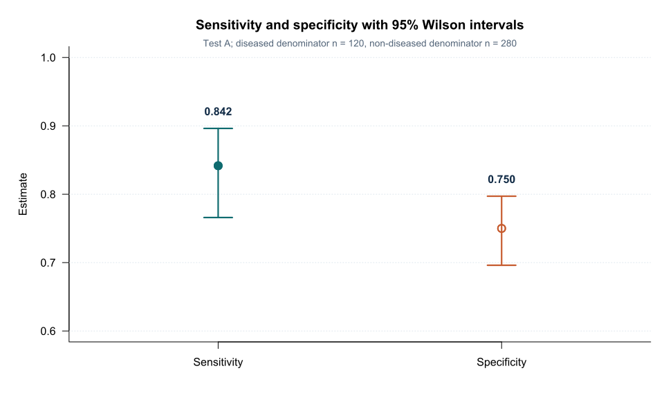
The figure should not imply that sensitivity and specificity are measured from the same denominator.

Threshold dependence

For a test where higher scores indicate disease:

• lowering the threshold usually increases sensitivity;
• lowering the threshold usually decreases specificity;
• raising the threshold usually has the opposite effect.

Sensitivity and specificity reported without the threshold are incomplete.

Spectrum effects

Sensitivity can increase when diseased participants have advanced, obvious disease.

Specificity can decrease when non-diseased participants have alternative conditions that mimic the target condition.

Accuracy estimated from healthy controls and severe cases may not apply to patients with diagnostic uncertainty.

Verification and review bias

If the reference standard is applied selectively, missed disease can be hidden.

If index-test interpreters know the reference result, interpretation may become more favourable.

STARD requires reporting of participant selection, test execution, blinding and handling of missing or indeterminate results [2].

Interpreting the output

Presenting the results

Suggested reporting

Report numerator, denominator, threshold, estimate, confidence interval, participant spectrum and intended clinical role.

Avoid vague statements such as “good sensitivity” without a prespecified acceptable range.

Common mistakes

Knowledge check

What is the sensitivity denominator?

Answer and reasoning

All participants with the target condition: true positives plus false negatives.

What is the false-positive rate?

Answer and reasoning

One minus specificity.

Does 84.2% sensitivity mean 84.2% of positive tests are diseased?

Answer and reasoning

No. That is the positive predictive value.

Why can sensitivity change between settings?

Answer and reasoning

Disease severity, patient spectrum, prior testing and execution can differ.

Why use Wilson intervals?

Answer and reasoning

They generally provide more reliable binomial coverage than simple Wald intervals.

Key take-home messages

References

1. Altman DG, Bland JM. Diagnostic tests 1: sensitivity and specificity. BMJ. 1994;308(6943):1552. https://doi.org/10.1136/bmj.308.6943.1552
2. Cohen JF, Korevaar DA, Altman DG, Bruns DE, Gatsonis CA, Hooft L, et al. STARD 2015 guidelines for reporting diagnostic accuracy studies: explanation and elaboration. BMJ Open. 2016;6:e012799. https://doi.org/10.1136/bmjopen-2016-012799
3. Wilson EB. Probable inference, the law of succession, and statistical inference. J Am Stat Assoc. 1927;22(158):209–212. https://doi.org/10.1080/01621459.1927.10502953
4. Brown LD, Cai TT, DasGupta A. Interval estimation for a binomial proportion. Stat Sci. 2001;16(2):101–133. https://doi.org/10.1214/ss/1009213286