Multiple Linear Regression

Overview

Multiple linear regression models a numerical outcome using two or more predictors.

Each coefficient is interpreted while holding the other included predictors fixed. The term adjusted describes model conditioning; it does not guarantee causal validity.

Why this matters

Clinical outcomes depend on several characteristics. Collinearity can make individual coefficients unstable [1], while excessive candidate complexity can cause overfitting [2]. Model specification should therefore follow the research objective and clinical knowledge [3].

When to use this method

Use multiple linear regression when the outcome is numerical, several predictors or adjustment variables are required and the conditional mean model is appropriate.

It does not automatically solve non-linearity, interaction, missing data, clustering, measurement error or unmeasured confounding.

Research question and variables

Data structure

Predictor coding

simulated data

Predictor	Coding	Interpretation unit
Baseline blood pressure	Numerical	1 mmHg
Telemonitoring	1 versus 0	Telemonitoring minus usual care
Age	Numerical	1 year
BMI	Numerical	1 kg/m²
Adherence	Numerical score	1 score unit
Male	1 versus 0	Male minus female

Statistical assumptions

How the method works

All coefficients are estimated simultaneously by minimising squared residuals.

Adjusted $R^2$ summarises in-sample outcome variation explained with a small penalty for model complexity. It does not assess causality or external validity.

Roles of variables in an adjusted model

Predictors can enter a model for different reasons:

• a primary exposure or treatment whose coefficient answers the main question;
• a confounder included to improve comparability;
• a prognostic variable included to improve precision;
• a design variable such as a stratification factor;
• an effect modifier represented through an interaction;
• a predictor used for individual prediction.

These roles should be decided from the study objective. A variable should not be described as a confounder merely because adding it changes a coefficient by an arbitrary percentage.

Coding categorical predictors

A binary predictor needs one indicator coefficient. A categorical predictor with $k$ levels usually needs $k-1$ indicators. Each coefficient compares one category with the stated reference while holding the other model variables fixed.

Changing the reference category changes coefficient labels but not fitted values. For an unordered exposure with several clinically relevant categories, planned contrasts can compare any pair without repeatedly refitting conceptually different models.

Interpreting continuous predictors

A continuous coefficient assumes a constant adjusted mean difference per unit across the represented range. One BMI unit may be clinically small, so reporting a five-unit contrast can be more readable:

$$5\beta_{\text{BMI}}$$

The scale should be selected before examining results. Standardising every predictor to one standard deviation can facilitate numerical comparison but hides clinical units and makes estimates population-dependent.

Adjustment and conditional interpretation

Holding other predictors fixed is a mathematical condition. It may describe an unrealistic comparison if two predictors are tightly linked. For example, comparing two people with the same baseline blood pressure but very different ages may represent a restricted subgroup rather than a population-average age effect.

Adjusted coefficients also depend on which variables are included. Adding a mediator can remove part of a treatment effect, while adjusting for a collider can introduce bias. The model formula therefore encodes scientific assumptions rather than merely controlling for more variables.

Assessing overall fit

The residual standard error remains an outcome-scale measure of unexplained variation. $R^2$ and adjusted $R^2$ summarise in-sample fit, but they should be accompanied by residual diagnostics and coefficient uncertainty.

An overall F test evaluates whether the selected slope parameters are all zero under the linear model. It does not show that every included predictor is necessary or that the model is well calibrated for prediction.

Missing data and analysis population

A complete-record regression uses only participants with observed values for every included variable. Adding one predictor with substantial missingness can change both the sample and the coefficient, making comparisons between models difficult.

Report the number included, reasons for exclusion and the missing-data method. Multiple imputation may be appropriate when its assumptions are defensible, but imputation does not repair measurement error or unmeasured confounding.

Worked example

Reproducible R analysis

make_hypertension_data <- function(n = 180) {
  set.seed(4583)
  i <- seq_len(n)

  data <- data.frame(
    participant_id = sprintf("H%03d", i),
    age = round(runif(n, 30, 80)),
    male = rbinom(n, 1, 0.5),
    bmi = pmin(pmax(round(rnorm(n, 27, 3.5), 1), 18), 40),
    physical_activity = round(runif(n, 2, 7), 1),
    telemonitoring = rbinom(n, 1, 0.5)
  )

  data$adherence <- 4 + runif(n, 0, 5) -
    0.015 * (data$age - 55) + 0.4 * data$telemonitoring
  data$baseline_sbp <- 92 + 0.52 * data$age + 0.85 * data$bmi +
    2.8 * data$male - 1.3 * data$physical_activity + rnorm(n, 0, 4)
  data$followup_sbp <- 58 + 0.47 * data$baseline_sbp +
    0.10 * data$age + 0.52 * data$bmi - 2.0 * data$adherence +
    2.0 * data$male - 4.5 * data$telemonitoring -
    0.55 * data$telemonitoring * (data$bmi - 27) +
    0.006 * (data$age - 55)^2 + rnorm(n, 0, 5)

  data
}

hypertension <- make_hypertension_data()

fit <- lm(
  followup_sbp ~ baseline_sbp + telemonitoring +
    age + bmi + adherence + male,
  data = hypertension
)

summary(fit)
confint(fit)

Cleaned R output

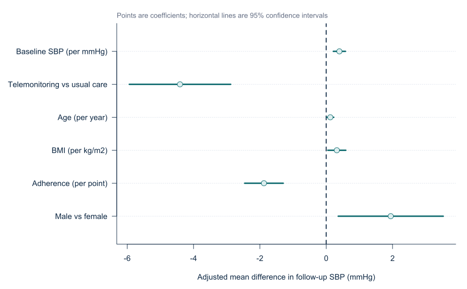
Predictor             Coefficient   95% CI
Baseline SBP             0.398      0.214 to 0.581
Telemonitoring          -4.409     -5.936 to -2.881
Age                      0.123      0.019 to 0.227
BMI                      0.320      0.050 to 0.590
Adherence               -1.877     -2.458 to -1.296
Male versus female       1.946      0.363 to 3.528

Base R uses lm() for this model [4].

Interpreting the output

Multicollinearity

Collinearity can produce unstable coefficients and large standard errors. Variance inflation factors are useful diagnostics but should not be treated using rigid universal thresholds [1].

Presenting the results

Present adjusted coefficients with units, reference categories and 95% confidence intervals in one coherent table.

Visualising adjusted coefficients

Suggested reporting

Overfitting MMed extension

Adding many candidate parameters can produce optimistic fit and unstable coefficients. Planning and validation are preferable to arbitrary automated selection [2], [3].

Common mistakes

Knowledge check

What does the telemonitoring coefficient represent?

Answer and reasoning

It is the adjusted mean follow-up difference conditional on the other included predictors and model form.

Does including age guarantee adequate confounding control?

Answer and reasoning

No. Measurement, functional form and unmeasured confounders still matter.

Why can correlated predictors have large standard errors?

Answer and reasoning

Their overlapping information makes separate conditional effects difficult to estimate.

Should a confounder be removed because p = 0.20?

Answer and reasoning

Not solely for that reason. Confounder selection should follow subject knowledge and the estimand.

What does adjusted R squared describe?

Answer and reasoning

It summarises in-sample fit with a complexity penalty, not causality or transportability.

Key take-home messages

References

1. O’Brien RM. A caution regarding rules of thumb for variance inflation factors. Qual Quant. 2007;41:673–690. https://doi.org/10.1007/s11135-006-9018-6
2. Babyak MA. What you see may not be what you get: a brief, nontechnical introduction to overfitting in regression-type models. Psychosom Med. 2004;66(3):411–421. https://doi.org/10.1097/01.psy.0000127692.23278.a9
3. Harrell FE Jr. Regression modeling strategies. 2nd ed. Cham: Springer; 2015. https://doi.org/10.1007/978-3-319-19425-7
4. R Core Team. Fitting linear models. R documentation, package stats version 4.6.1. Vienna: R Foundation for Statistical Computing; 2026. https://stat.ethz.ch/R-manual/R-devel/library/stats/html/lm.html