
Part 11 · Module 3
Predictive Values
Learn how positive and negative predictive values translate test results into post-test disease probabilities and why they change with prevalence and setting.
Learning outcomes
After completing this lecture, you should be able to:
- Calculate positive and negative predictive values from a 2 × 2 table.
- Identify the correct test-result denominators.
- Interpret predictive values as post-test probabilities in the study population.
- Explain how prevalence and patient selection affect predictive values.
- Use Bayes' theorem to calculate predictive values at alternative prevalences.
- Use R code to report predictive values with confidence intervals.
Overview
Predictive values answer the clinical questions that follow a test result.
Positive predictive value asks:
Among participants with a positive test, what proportion have the target condition?
Negative predictive value asks:
Among participants with a negative test, what proportion do not have the target condition?
They condition on the observed test result.
Predictive values depend on:
- test sensitivity;
- test specificity;
- target-condition prevalence;
- participant spectrum;
- verification and follow-up.
They should not be transported unchanged to a population with a different pre-test probability [1].
Why this matters
A screening test can have high sensitivity and specificity but a modest positive predictive value when disease is uncommon.
Conversely, a negative result may be highly reassuring in a low-prevalence population but less reassuring in a specialist referral population.
Predictive values are therefore properties of the test in a population and pathway, not the test alone. Formal diagnostic-study methods and transport considerations are reviewed by Zhou and colleagues [2].
When to use these measures
Use predictive values when the study sample reflects the population in which the test result will be interpreted.
They are especially useful for:
- communicating post-test probability;
- counselling after positive or negative screening;
- estimating referral burden;
- planning confirmatory testing.
Case–control diagnostic studies with investigator-selected numbers of diseased and non-diseased participants cannot estimate clinically applicable predictive values directly. STARD requires recruitment and participant-flow details that allow this limitation to be assessed [3].
Research question and variables
The false-discovery proportion among positive tests is:
The false-omission proportion among negative tests is:
Data structure
Test-result denominators
simulated data| Test-result group | Condition present | Condition absent | Total |
|---|---|---|---|
| Positive | 101 | 70 | 171 |
| Negative | 19 | 210 | 229 |
PPV is calculated across the positive row. NPV is calculated across the negative row.
Statistical assumptions
Worked example
Bayes’ theorem and prevalence
Given sensitivity , specificity and prevalence :
Using Test A sensitivity and specificity:
| Prevalence | PPV | NPV |
|---|---|---|
| 5% | 15.1% | 98.9% |
| 10% | 27.2% | 97.7% |
| 30% | 59.1% | 91.7% |
| 60% | 83.5% | 75.9% |
The same test characteristics produce very different predictive values.
Worked analysis in R
make_diagnostic_data <- function(n = 400) {
  id <- seq_len(n)
  age <- 20 + ((7 * id) %% 61)
  male <- as.integer(id %% 2 == 0)

  disease <- as.integer(
    ((id * 37) %% 100) < 30
  )

  score_a <-
    47 +
    11 * disease +
    0.08 * (age - 50) +
    7.5 * sin(id * 1.13) +
    3.5 * cos(id * 0.37)

  score_b <-
    48 +
    9 * disease +
    0.05 * (age - 50) +
    7.2 * sin(id * 1.13 + 0.45) +
    4.0 * cos(id * 0.37 + 0.20)

  disease_rank <- (id * 43) %% 100
  nondisease_rank <- (id * 47) %% 100

  reference_positive <- ifelse(
    disease == 1,
    disease_rank < 88,
    nondisease_rank >= 95
  )

  data.frame(
    id = id,
    age = age,
    male = male,
    disease = disease,
    score_a = score_a,
    score_b = score_b,
    reference_positive = as.integer(
      reference_positive
    )
  )
}

diagnostic_data <- make_diagnostic_data()

cutoff_a <- 51.962318662698785
cutoff_b <- 55.26626112612387

diagnostic_data$test_a_positive <- as.integer(
  diagnostic_data$score_a >= cutoff_a
)

diagnostic_data$test_b_positive <- as.integer(
  diagnostic_data$score_b >= cutoff_b
)

diagnostic_table <- with(
  diagnostic_data,
  table(
    test_a_positive,
    disease
  )
)

tn <- diagnostic_table["0", "0"]
fn <- diagnostic_table["0", "1"]
fp <- diagnostic_table["1", "0"]
tp <- diagnostic_table["1", "1"]

wilson_ci <- function(successes, total, conf.level = 0.95) {
  z <- qnorm(
    1 - (1 - conf.level) / 2
  )

  estimate <- successes / total
  denominator <- 1 + z^2 / total

  centre <- (
    estimate +
    z^2 / (2 * total)
  ) / denominator

  half_width <- (
    z / denominator
  ) *
    sqrt(
      estimate *
        (1 - estimate) / total +
      z^2 / (4 * total^2)
    )

  c(
    estimate = estimate,
    lower = centre - half_width,
    upper = centre + half_width
  )
}

ppv <- wilson_ci(
  tp,
  tp + fp
)

npv <- wilson_ci(
  tn,
  tn + fn
)

predictive_values <- function(
  prevalence,
  sensitivity,
  specificity
) {
  positive_predictive_value <-
    sensitivity * prevalence /
    (
      sensitivity * prevalence +
      (1 - specificity) *
        (1 - prevalence)
    )

  negative_predictive_value <-
    specificity *
    (1 - prevalence) /
    (
      (1 - sensitivity) *
        prevalence +
      specificity *
        (1 - prevalence)
    )

  data.frame(
    prevalence = prevalence,
    ppv = positive_predictive_value,
    npv = negative_predictive_value
  )
}

prevalence_grid <- seq(
  0.01,
  0.70,
  by = 0.01
)

curve_data <- predictive_values(
  prevalence_grid,
  sensitivity = 101 / 120,
  specificity = 210 / 280
)

rbind(
  ppv = ppv,
  npv = npv
)
Selected analysis output
Measure   Estimate   95% CI
PPV         0.591    0.516 to 0.662
NPV         0.917    0.874 to 0.946
Visualising prevalence effects
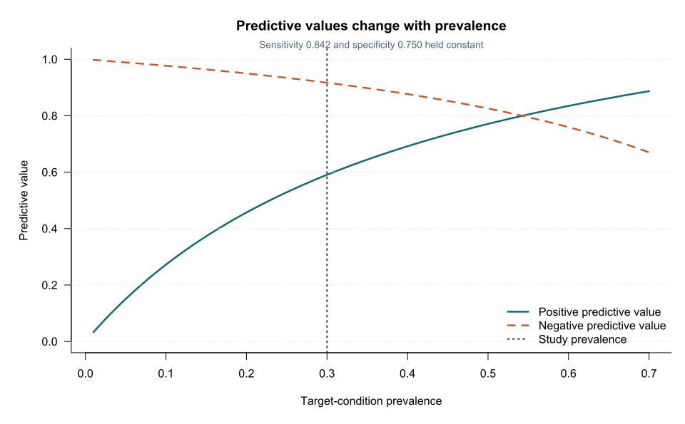
The curves assume sensitivity and specificity remain constant across populations.
In reality, changes in prevalence often accompany changes in disease spectrum, which can also alter sensitivity and specificity [4].
Pre-test probability
Prevalence is a population-average pre-test probability.
For an individual patient, pre-test probability may also depend on:
- symptoms;
- age;
- risk factors;
- prior tests;
- referral setting;
- clinician assessment.
Predictive values calculated from a broad study prevalence may not match a specific patient.
Case–control designs
In a case–control accuracy study, investigators choose the numbers of cases and controls.
The sample disease proportion is artificial.
Sensitivity and specificity can sometimes be estimated, but sample PPV and NPV should not be interpreted as clinical post-test probabilities.
Interpreting the output
Presenting the results
Suggested reporting
Report the study prevalence, recruitment setting, numerator, denominator, confidence interval and intended population.
If transporting predictive values, state the assumed sensitivity, specificity and target prevalence.
Common mistakes
Knowledge check
What is the PPV denominator?
Answer and reasoning
All participants with a positive index test: true positives plus false positives.
Why does PPV usually fall in low-prevalence settings?
Answer and reasoning
False positives can outnumber true positives when the target condition is uncommon.
Can a case–control sample estimate clinical PPV directly?
Answer and reasoning
No. The case–control disease proportion is determined by the investigators.
What does NPV 91.7% mean?
Answer and reasoning
Among negative tests in this study, 91.7% did not have the target condition.
Why might transported PPV differ even after adjusting prevalence?
Answer and reasoning
Sensitivity and specificity can also change because the patient spectrum and test execution differ.
Key take-home messages
References
- Altman DG, Bland JM. Diagnostic tests 2: predictive values. BMJ. 1994;309(6947):102. https://doi.org/10.1136/bmj.309.6947.102
- Zhou XH, Obuchowski NA, McClish DK. Statistical methods in diagnostic medicine. 2nd ed. Hoboken (NJ): Wiley; 2011. https://doi.org/10.1002/9780470906514
- Bossuyt PM, Reitsma JB, Bruns DE, Gatsonis CA, Glasziou PP, Irwig L, et al. STARD 2015: an updated list of essential items for reporting diagnostic accuracy studies. BMJ. 2015;351:h5527. https://doi.org/10.1136/bmj.h5527
- Leeflang MMG, Rutjes AWS, Reitsma JB, Hooft L, Bossuyt PMM. Variation of a test’s sensitivity and specificity with disease prevalence. CMAJ. 2013;185(11):E537–E544. https://doi.org/10.1503/cmaj.121286
These notes support learning and research planning and do not replace statistical consultation for a specific study.