Latent-Variable Analysis and Structural Equation Modelling

Overview

Structural equation modelling, SEM, combines:

• latent-variable measurement models;
• regression-like structural relations;
• correlated disturbances;
• direct and indirect effects.

Confirmatory factor analysis, CFA, is the measurement-model component.

SEM is not automatically causal.

Causal interpretation depends on design, temporal ordering and assumptions.

Why this matters

Observed questionnaire totals contain measurement error.

Latent-variable models can represent shared construct variance and item-specific error.

However, complex models can fit superficially while being unidentified, overfitted or substantively implausible.

When to use SEM

Use SEM when:

• latent constructs are central;
• multiple indicators are available;
• measurement error must be modelled;
• a confirmatory structural theory exists;
• sample size and data quality support the parameters.

Do not use SEM solely to obtain many paths in one figure.

Research question and variables

Measurement equations are:

$$x_j=\lambda_j\xi+\varepsilon_j$$

Structural equations are:

The indirect effect is:

$$\gamma_1\beta$$

Data structure

SEM indicators

simulated data

Latent construct	Indicators
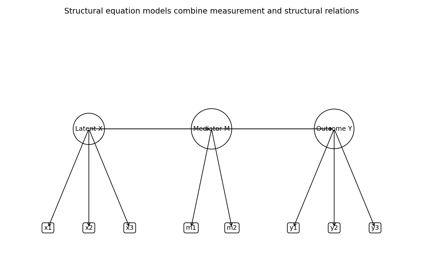
X	x1, x2, x3
M	m1, m2
Y	y1, y2, y3

Two-indicator factors require additional constraints and strong justification.

Statistical assumptions

Identification and scaling

A latent factor has no natural unit.

Common scaling methods are:

• fix one loading to 1;
• fix latent variance to 1.

Identification requires enough unique observed information for all free parameters.

Estimation

For approximately continuous normal indicators, maximum likelihood is common.

For ordinal items, WLSMV is often appropriate.

Robust ML can address non-normality.

Estimator choice changes assumptions and fit statistics.

Worked example

Worked analysis in R

sem_data <- read.csv(
  "data/part-16-sem-data.csv"
)

library(lavaan)

sem_model <- '
  X =~ x1 + x2 + x3
  M =~ m1 + m2
  Y =~ y1 + y2 + y3

  M ~ a * X
  Y ~ b * M + c_direct * X

  indirect := a * b
  total := c_direct + indirect
'

sem_fit <- sem(
  sem_model,
  data = sem_data,
  estimator = "MLR",
  missing = "fiml"
)

summary(
  sem_fit,
  standardized = TRUE,
  fit.measures = TRUE,
  rsquare = TRUE
)

modindices(
  sem_fit,
  sort. = TRUE
)

Selected analysis output

The simulated indicators load strongly on their intended latent variables.

The X-to-M, M-to-Y and X-to-Y paths are detectable in the expected directions.

Visualising the SEM

Model fit

Common indices include:

• chi-square;
• CFI;
• TLI;
• RMSEA;
• SRMR.

No universal cutoff proves adequacy.

Fit should be evaluated using:

• theory;
• residuals;
• parameter plausibility;
• alternative models;
• replication.

Modification indices

Modification indices estimate potential fit improvement from freeing parameters.

Data-driven residual correlations can overfit.

Every modification should have substantive rationale and ideally be validated in new data.

Measurement invariance

Before comparing latent means across groups or time, examine:

• configural invariance;
• metric invariance;
• scalar invariance;
• residual invariance when relevant.

Without scalar invariance, latent mean comparisons may be biased.

Interpreting the output

Presenting the analysis

Suggested reporting

Report model diagram, syntax, identification, estimator, missing data, fit indices, loadings, residuals, standardised and unstandardised paths, indirect effects and modifications [1], [2].

Confirmatory factor-analysis practice and the limitations of universal fit-index cut-offs are discussed by Brown and by Hu and Bentler [3], [4].

Common mistakes

Knowledge check

What is a latent variable?

Answer and reasoning

An unobserved construct represented through relationships among observed indicators.

Why set the latent scale?

Answer and reasoning

The construct has no natural numerical unit without a constraint.

What does WLSMV suit?

Answer and reasoning

Many ordinal-indicator CFA and SEM applications.

Does good fit prove the causal model?

Answer and reasoning

No.

Why test invariance?

Answer and reasoning

To support comparable construct meaning across groups or time.

Key take-home messages

References

1. Rosseel Y. lavaan: an R package for structural equation modeling. J Stat Softw. 2012;48(2):1–36. https://doi.org/10.18637/jss.v048.i02
2. Kline RB. Principles and practice of structural equation modeling. 5th ed. New York: Guilford; 2023.
3. Brown TA. Confirmatory factor analysis for applied research. 2nd ed. New York: Guilford; 2015.
4. Hu LT, Bentler PM. Cutoff criteria for fit indexes. Struct Equ Modeling. 1999;6(1):1–55. https://doi.org/10.1080/10705519909540118