Spatial and Geographical Health Data

Overview

Spatial health data contain location.

Common forms are:

• geocoded points;
• administrative areas;
• healthcare networks;
• environmental rasters;
• travel paths.

Nearby areas can be more similar than distant areas.

Ordinary independence assumptions may fail.

Why this matters

Maps can reveal geographic variation but can also mislead through:

• unstable small-area rates;
• arbitrary boundaries;
• population differences;
• multiple testing;
• visual colour choices;
• disclosure risk.

Spatial analysis should combine maps with uncertainty and substantive context.

When to use spatial analysis

Use spatial methods when location is part of the research question:

• disease mapping;
• access to care;
• environmental exposure;
• cluster detection;
• service planning;
• spatial prediction.

Do not add maps merely for decoration.

Research question and variables

Area rate is:

$$r_i= \frac{y_i}{N_i}$$

Spatial autocorrelation asks whether neighbouring values are more alike than expected.

Moran’s I is:

Data structure

Area-level spatial data

simulated data

Variable	Meaning
area	Geographic unit
population	Denominator
cases	Event count
rate_per_1000	Crude area rate
Geometry	Polygon boundary
Neighbours	Spatial weights

Statistical assumptions

Rate instability

Small populations produce highly variable crude rates.

Options include:

• exact intervals;
• empirical Bayes smoothing;
• hierarchical Poisson models;
• age standardisation;
• aggregation.

Smoothing should not erase real local variation or conceal uncertainty.

Worked example

Worked analysis in R

spatial_data <- read.csv(
  "data/part-16-spatial-data.csv"
)

spatial_data$rate_per_1000 <- (
  spatial_data$cases /
  spatial_data$population *
  1000
)

# A real analysis would read geometries:
# library(sf)
# areas <- st_read("areas.gpkg")
# map_data <- merge(
#   areas,
#   spatial_data,
#   by = "area"
# )

# Neighbour weights:
# library(spdep)
# nb <- poly2nb(map_data)
# listw <- nb2listw(nb)
# moran.test(
#   map_data$rate_per_1000,
#   listw
# )

Selected analysis output

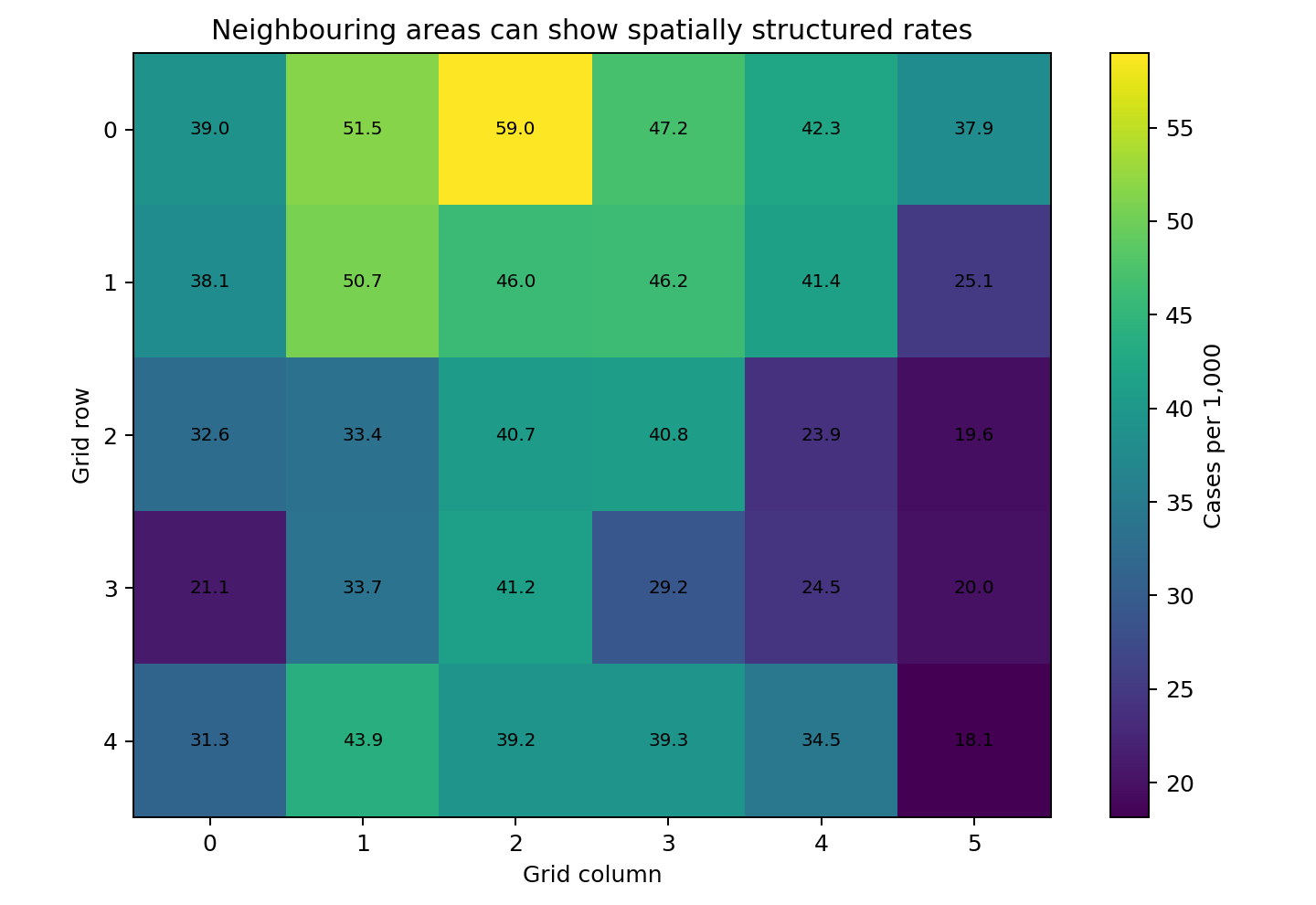
The simulated grid contains 30 areas with spatially patterned rates.

A real Moran's I requires polygon geometry and a prespecified neighbour definition.

Visualising spatial rates

Ecological fallacy

An area-level association does not establish the same individual-level association.

The modifiable areal unit problem means results can change when boundaries or aggregation scales change.

Spatial regression

Models include:

• conditional autoregressive models;
• simultaneous autoregressive models;
• spatial lag models;
• spatial error models;
• Gaussian processes;
• geographically weighted regression.

Method choice depends on whether spatial structure lies in outcome, residuals or relationships.

Cluster detection

Methods such as scan statistics search for local excess risk.

Clusters should be interpreted with:

• multiple-testing correction;
• population at risk;
• surveillance bias;
• pre-existing hypotheses.

Interpreting the output

Presenting the analysis

Suggested reporting

Report geography, coordinate system, geocoding, denominator, standardisation, spatial weights, model, uncertainty, privacy and scale sensitivity [1], [2].

Hierarchical disease-mapping models and public-health spatial-statistics methods are developed by Besag and colleagues and by Waller and Gotway [3], [4].

Common mistakes

Knowledge check

What does spatial autocorrelation mean?

Answer and reasoning

Nearby observations are more similar or dissimilar than expected under independence.

Why are small-area rates unstable?

Answer and reasoning

Small denominators produce large sampling variation.

What is ecological fallacy?

Answer and reasoning

Inferring individual-level relationships from area-level associations.

Why does neighbour definition matter?

Answer and reasoning

It determines which observations are treated as spatially connected.

What should accompany a disease map?

Answer and reasoning

Denominators, uncertainty, standardisation and privacy safeguards.

Key take-home messages

References

1. Pebesma E. Simple features for R: standardized support for spatial vector data. R J. 2018;10(1):439–446. https://doi.org/10.32614/RJ-2018-009
2. Bivand RS, Pebesma E, Gómez-Rubio V. Applied spatial data analysis with R. 2nd ed. New York: Springer; 2013.
3. Besag J, York J, Mollié A. Bayesian image restoration with applications in spatial statistics. Ann Inst Stat Math. 1991;43:1–20. https://doi.org/10.1007/BF00116466
4. Waller LA, Gotway CA. Applied spatial statistics for public health data. Hoboken: Wiley; 2004.