Longitudinal Data Analysis

Overview

Longitudinal data contain repeated observations ordered through time for the same independent units.

They allow researchers to study mean change, differences in trajectories, individual heterogeneity, time-varying exposures and the timing of missing observations.

Longitudinal analysis is more than performing separate tests at each visit. The mean profile, covariance, missing-data process and estimand must be considered together [1], [2].

Why this matters

A trial can show similar baseline means, a modest difference at month 3 and a larger difference at month 6.

One overall group effect cannot represent this changing contrast. A single baseline-to-final change score also discards the intermediate trajectory and can exclude participants with partial follow-up.

When to use this framework

Use longitudinal analysis when the same outcome is recorded at ordered times, timing is scientifically important, incomplete visits occur, or participant-specific trajectories matter.

A paired t-test may be adequate for exactly two complete measurements and one mean-change estimand, but it does not generalise naturally to richer trajectories. Modern longitudinal modelling generally offers greater flexibility than classical complete-case repeated-measures ANOVA [3].

Research question and variables

Possible estimands include:

• mean outcome at each visit;
• month-6 group difference;
• average group difference over follow-up;
• difference in slopes;
• area under the mean curve;
• probability of response over time;
• subject-specific change rate.

The model should be chosen after the estimand is defined.

Data structure

Essential longitudinal variables

simulated data

Table 1. Long-format variables

Variable	Role
id	Participant identifier
group	Time-invariant treatment
month	Repeated time
sbp	Repeated numerical outcome
age	Time-invariant covariate
medication_dose	Example time-varying covariate
visit_observed	Visit-completion indicator

Long format is generally preferable for GEE, mixed-effects models, irregular timing, time-varying predictors and trajectory plots.

Statistical assumptions

How to represent time

Categorical time

Categorical time estimates a separate mean at each scheduled visit and imposes no linear trend.

Continuous time

A continuous linear term estimates one constant slope and can use actual visit timing.

Non-linear time

Polynomial, spline or piecewise functions can represent curved or phase-specific trajectories.

Observed mean profiles

Observed systolic blood-pressure means

simulated data

Table 2. Mean (SD) by group and visit

Group	Baseline	Month 3	Month 6
Usual care	151.9 (6.6)	147.2 (6.9)	142.8 (6.8)
Telemonitoring	151.0 (6.2)	144.2 (6.3)	137.5 (6.8)

Note: Each cell contains 60 simulated observations.

Observed telemonitoring-minus-usual-care differences are −0.9, −3.1 and −5.3 mmHg across the three visits.

Worked example

Worked analysis in R

make_longitudinal_data <- function(n = 120) {
  records <- vector("list", n * 3)
  row_number <- 1

  for (participant_id in seq_len(n)) {
    group <- as.integer(participant_id %% 2 == 0)
    age <- 35 + ((7 * participant_id) %% 41)
    male <- as.integer(participant_id %% 3 == 0)

    random_intercept <-
      7 * sin(participant_id * 0.71) +
      3 * cos(participant_id * 0.19)

    random_slope <-
      0.45 * sin(participant_id * 0.37)

    for (month in c(0, 3, 6)) {
      residual <-
        3.5 * sin(participant_id * 1.13 + month * 0.91) +
        1.2 * cos(participant_id * 0.23 + month * 0.33)

      sbp <-
        151 +
        0.18 * (age - 55) +
        1.8 * male +
        random_intercept -
        1.5 * month -
        0.4 * group -
        0.75 * group * month +
        random_slope * month +
        residual

      records[[row_number]] <- data.frame(
        id = participant_id,
        group = group,
        age = age,
        male = male,
        month = month,
        sbp = sbp
      )

      row_number <- row_number + 1
    }
  }

  longitudinal <- do.call(rbind, records)

  longitudinal$group <- factor(
    longitudinal$group,
    levels = c(0, 1),
    labels = c("Usual care", "Telemonitoring")
  )

  longitudinal <- longitudinal[
    order(longitudinal$id, longitudinal$month),
  ]

  rownames(longitudinal) <- NULL
  longitudinal
}

longitudinal <- make_longitudinal_data()

observed_summary <- aggregate(
  sbp ~ group + month,
  data = longitudinal,
  FUN = function(x) {
    c(
      n = length(x),
      mean = mean(x),
      sd = sd(x),
      se = sd(x) / sqrt(length(x))
    )
  }
)

observed_summary

observed_means <- observed_summary$sbp[, "mean"]
observed_ses <- observed_summary$sbp[, "se"]
observed_limits <- range(
  observed_means - 1.96 * observed_ses,
  observed_means + 1.96 * observed_ses
)
axis_padding <- diff(observed_limits) * 0.06

plot(
  NA,
  xlim = c(-0.25, 6.25),
  ylim = observed_limits + c(-axis_padding, axis_padding),
  xlab = "Month",
  ylab = "Mean systolic blood pressure (mmHg)",
  xaxt = "n"
)

axis(1, at = c(0, 3, 6))

for (group_name in levels(longitudinal$group)) {
  subset_data <- longitudinal[
    longitudinal$group == group_name,
  ]

  means <- tapply(
    subset_data$sbp,
    subset_data$month,
    mean
  )

  lines(
    c(0, 3, 6),
    means,
    type = "b"
  )
}

legend(
  "topright",
  legend = levels(longitudinal$group),
  lty = 1,
  pch = 1
)

Selected analysis output

Group             Month  Mean SBP   SD
Usual care           0     151.9    6.6
Usual care           3     147.2    6.9
Usual care           6     142.8    6.8
Telemonitoring       0     151.0    6.2
Telemonitoring       3     144.2    6.3
Telemonitoring       6     137.5    6.8

Visualising longitudinal patterns

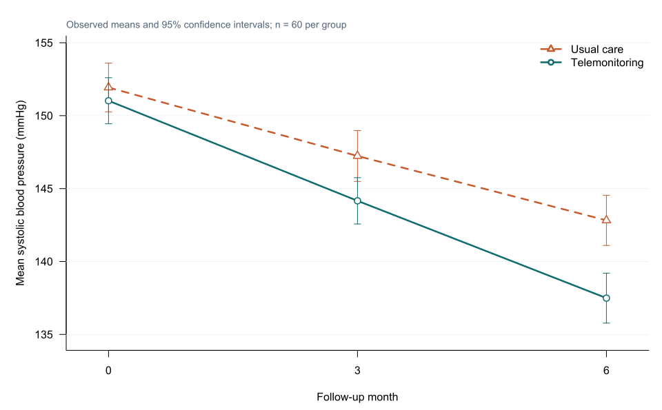
Useful graphics include individual trajectories, group mean profiles with intervals, visit-specific distributions and missingness plots.

Missing longitudinal data

Missingness can be intermittent or monotone dropout and can depend on observed or unobserved outcomes.

Repeated-measures ANOVA usually uses complete participants. Mixed models and GEE use incomplete data differently, but neither is automatically unbiased under every missingness mechanism.

Time-varying covariates

A time-varying predictor can combine between-person and within-person information.

Medication dose, for example, may be higher in generally sicker participants and may also rise after individual worsening. Interpretation can require person-mean centring, lagging or causal longitudinal methods.

Choosing an analysis

Interpreting the output

Presenting the results

Suggested reporting

Report the number observed at each visit, time scale, interaction terms, covariance or random-effects structure, marginal or subject-specific interpretation, missing-data assumptions and clinically important contrasts [1], [2]. Practical epidemiological interpretation is developed further by Twisk [4].

Common mistakes

Knowledge check

What does a group-by-time interaction estimate?

Answer and reasoning

It estimates how the group difference changes with time on the model scale.

Why can separate visit tests be problematic?

Answer and reasoning

They do not estimate one coherent trajectory effect and create multiple testing.

When is categorical time preferable?

Answer and reasoning

When visit-specific means are important or a simple slope is not credible.

Does a mixed model make missing outcomes ignorable automatically?

Answer and reasoning

No. Validity still depends on the likelihood model and missingness assumptions.

Why plot observed profiles before modelling?

Answer and reasoning

They reveal trajectory shape, variability, group separation and missingness patterns.

Key take-home messages

References

1. Diggle PJ, Heagerty P, Liang KY, Zeger SL. Analysis of longitudinal data. 2nd ed. Oxford: Oxford University Press; 2002. https://doi.org/10.1093/oso/9780198524847.001.0001
2. Fitzmaurice GM, Laird NM, Ware JH. Applied longitudinal analysis. 2nd ed. Hoboken (NJ): Wiley; 2011.
3. Gueorguieva R, Krystal JH. Move over ANOVA: progress in analyzing repeated-measures data. Arch Gen Psychiatry. 2004;61(3):310–317. https://doi.org/10.1001/archpsyc.61.3.310
4. Twisk JWR. Applied longitudinal data analysis for epidemiology. 2nd ed. Cambridge: Cambridge University Press; 2013. https://doi.org/10.1017/CBO9781139342834