Regression Diagnostics

Overview

Regression diagnostics assess whether a fitted model represents the data sufficiently well for its intended use.

Important concepts are:

• residual: observed minus fitted outcome;
• outlier: observation unusual in the outcome direction;
• leverage: unusual predictor pattern;
• influence: degree to which an observation affects fitted results.

These properties are related but not identical.

Why this matters

A data error can distort coefficients. A valid extreme participant may reveal important population heterogeneity. Automatic deletion can introduce bias.

Diagnostics should trigger investigation, source verification and sensitivity analysis—not mechanical removal.

When to use this method

Diagnostics are required after fitting every regression model, with methods adapted to the model family.

They do not prove that assumptions are true. They identify patterns needing investigation.

Research question and variables

The fitted model uses follow-up blood pressure as outcome and baseline blood pressure, telemonitoring, age, BMI, adherence and sex as predictors.

Data structure

Diagnostic quantities

simulated data

Quantity	Main question
Residual	Is the observed outcome unusual given predictors?
Leverage	Is the predictor combination unusual?
Cook’s distance	Does the observation materially affect the fitted coefficients?
DFFITS	Does it materially affect its fitted value?

Statistical assumptions

How the method works

Cook’s distance combines residual magnitude and leverage.

Values such as $4/n$ are screening guides, not universal deletion thresholds [1].

Residual-versus-fitted plot

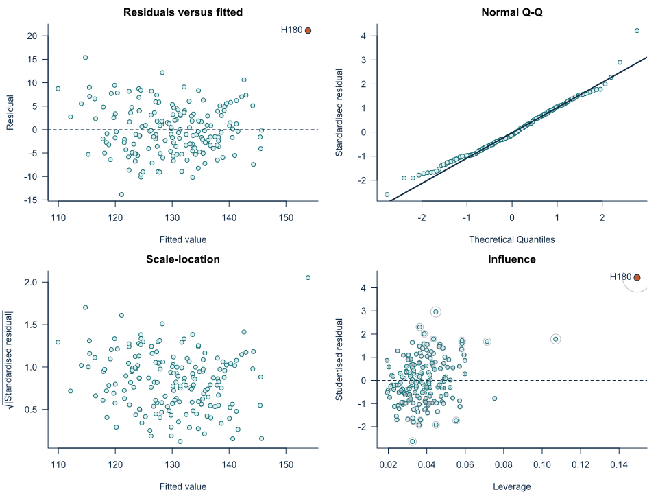
A random horizontal cloud around zero supports the mean-function and variance assumptions. Curvature suggests missing nonlinear terms. A funnel shape suggests non-constant variance. Distinct bands may arise from an omitted categorical predictor or outcome rounding.

The plot should be interpreted with the outcome and study design. Minor deviations in a large dataset may have little practical effect, whereas a systematic pattern affecting the primary contrast requires correction.

Normal quantile plot

A quantile–quantile plot compares residual ordering with a normal reference. Tail departures can indicate outliers or heavy-tailed residuals.

Normal residuals are most important for exact small-sample t and F inference. Large samples may support approximate inference despite moderate departures, but influential tail observations still require attention.

Leverage

Leverage depends only on predictor values under ordinary linear regression. An observation with an unusual combination of age, BMI and baseline blood pressure can have high leverage even when each variable alone is not extreme.

Average leverage equals $p/n$, where $p$ includes the intercept. Values around two or three times the average can be flagged for review, but no universal threshold defines an invalid observation.

Influence measures

Cook’s distance summarises the combined effect of residual and leverage on the fitted coefficient vector. DFBETAs describe influence on individual coefficients, while DFFITS describes influence on a fitted value.

An observation can strongly affect the treatment coefficient but have a modest overall Cook’s distance. Diagnostics should therefore focus on the primary estimand as well as global model change.

Heteroscedasticity

When residual variance changes with fitted values, ordinary least-squares coefficients can remain unbiased under correct mean specification, but conventional standard errors may be wrong.

Possible responses include:

• revising the mean function;
• transforming the outcome when scientifically meaningful;
• modelling the variance;
• using heteroscedasticity-consistent standard errors;
• reporting robust sensitivity analyses.

The chosen response should address the reason for the pattern rather than merely produce a desired p-value.

Sensitivity analysis

A useful sensitivity analysis compares:

• full-data estimates;
• estimates after correction of confirmed errors;
• estimates excluding a valid but highly influential observation;
• an alternative robust model where justified.

The primary result should follow the prespecified eligibility and data-quality rules. Sensitivity analyses demonstrate robustness rather than replace the main analysis selectively.

Diagnostics for other regression families

Logistic and count models use deviance or Pearson residuals and have model-specific checks for calibration, separation, dispersion and zero patterns. The general principles remain: examine mean structure, variance, influence and dependence using diagnostics appropriate to the model family.

Worked example

Reproducible R analysis

make_hypertension_data <- function(n = 180) {
  set.seed(4583)
  i <- seq_len(n)

  data <- data.frame(
    participant_id = sprintf("H%03d", i),
    age = round(runif(n, 30, 80)),
    male = rbinom(n, 1, 0.5),
    bmi = pmin(pmax(round(rnorm(n, 27, 3.5), 1), 18), 40),
    physical_activity = round(runif(n, 2, 7), 1),
    telemonitoring = rbinom(n, 1, 0.5)
  )

  data$adherence <- 4 + runif(n, 0, 5) -
    0.015 * (data$age - 55) + 0.4 * data$telemonitoring
  data$baseline_sbp <- 92 + 0.52 * data$age + 0.85 * data$bmi +
    2.8 * data$male - 1.3 * data$physical_activity + rnorm(n, 0, 4)
  data$followup_sbp <- 58 + 0.47 * data$baseline_sbp +
    0.10 * data$age + 0.52 * data$bmi - 2.0 * data$adherence +
    2.0 * data$male - 4.5 * data$telemonitoring -
    0.55 * data$telemonitoring * (data$bmi - 27) +
    0.006 * (data$age - 55)^2 + rnorm(n, 0, 5)

  data
}

hypertension <- make_hypertension_data()

diagnostic_data <- hypertension

diagnostic_data[
  diagnostic_data$participant_id == "H180",
  c("age", "bmi", "baseline_sbp", "followup_sbp")
] <- c(92, 38, 180, 175)

fit <- lm(
  followup_sbp ~ baseline_sbp + telemonitoring +
    age + bmi + adherence + male,
  data = diagnostic_data
)

diagnostics <- data.frame(
  participant_id = diagnostic_data$participant_id,
  leverage = hatvalues(fit),
  studentised_residual = rstudent(fit),
  cooks_distance = cooks.distance(fit),
  dffits = dffits(fit)
)

head(
  diagnostics[
    order(diagnostics$cooks_distance, decreasing = TRUE),
  ],
  5
)

par(mfrow = c(2, 2))
plot(fit)
par(mfrow = c(1, 1))

Cleaned R output

Participant   Leverage   Studentised residual   Cook's distance   DFFITS
H180           0.149             4.44                0.446          1.86
H095           0.045             2.96                0.056          0.64
H174           0.107             1.79                0.054          0.62

Base R provides influence.measures(), hatvalues(), rstudent() and cooks.distance() [2]. A complete diagnostic review considers residual form, leverage and influence together rather than relying on one threshold [3].

Interpreting the output

Presenting the results

Present material diagnostic findings, source verification and sensitivity analyses without using thresholds as deletion rules.

Visualising model diagnostics

Suggested reporting

Robust standard errors are not a universal repair MMed extension

Heteroscedasticity-robust standard errors can improve inference under variance misspecification, but they do not repair non-linearity, influential points, measurement error or an inappropriate estimand.

Common mistakes

Knowledge check

What is leverage?

Answer and reasoning

It measures how unusual an observation’s predictor values are relative to the rest of the dataset.

Can an outcome outlier have low influence?

Answer and reasoning

Yes. Influence depends on residual size, leverage and model structure.

Does Cook's distance above 4/n require deletion?

Answer and reasoning

No. It is a screening guide that prompts investigation.

What should happen before excluding a point?

Answer and reasoning

Verify source data, eligibility, units and clinical plausibility and assess model specification.

Why report sensitivity analysis?

Answer and reasoning

It shows whether conclusions depend materially on an influential but plausible observation.

Key take-home messages

References

1. Cook RD. Detection of influential observation in linear regression. Technometrics. 1977;19(1):15–18. https://doi.org/10.2307/1268249
2. R Core Team. Regression deletion diagnostics. R documentation, package stats version 4.6.1. Vienna: R Foundation for Statistical Computing; 2026. https://stat.ethz.ch/R-manual/R-devel/library/stats/html/influence.measures.html
3. Fox J, Weisberg S. An R companion to applied regression. 3rd ed. Thousand Oaks (CA): Sage; 2019.