Bayesian Statistics for Clinicians

Overview

Bayesian statistics updates prior information using observed data.

Bayes’ theorem gives:

where:

• $p(\theta)$ is the prior;
• $p(y\mid\theta)$ is the likelihood;
• $p(\theta\mid y)$ is the posterior.

The posterior supports direct probability statements about parameters under the model.

Why this matters

Clinicians often want answers such as:

• What is the probability treatment is beneficial?
• What is the probability benefit exceeds a clinical threshold?
• What is the probability one model is better?
• How should previous evidence inform a new trial?

Bayesian analysis can answer these questions explicitly.

When to use Bayesian methods

Useful settings include:

• sequential trials;
• small populations;
• external borrowing;
• diagnostic updating;
• hierarchical models;
• decision analysis;
• complex prediction models.

Bayesian methods do not remove the need for design, sensitivity analysis or transparent assumptions.

Research question and variables

The simulated treatment effect is negative when beneficial.

Prior:

$$\theta\sim N(0,1.5^2)$$

Likelihood estimate:

$$\hat\theta=-0.42,\quad SE=0.18$$

The posterior is normal under conjugacy.

Data structure

Bayesian analysis ingredients

simulated data

Component	Value
Prior mean	0
Prior SD	1.5
Data estimate	−0.42
Data SE	0.18
Clinical threshold	−0.20

Statistical assumptions

Conjugate normal updating

Posterior variance is:

$$V_{post} = \left( \frac{1}{V_{prior}}+ \frac{1}{V_{data}} \right)^{-1}$$

Posterior mean is a precision-weighted average:

$$\mu_{post} = V_{post} \left( \frac{\mu_{prior}}{V_{prior}}+ \frac{\hat\theta}{V_{data}} \right)$$

Worked example

Worked analysis in R

prior_mean <- 0
prior_sd <- 1.5

estimate <- -0.42
standard_error <- 0.18

posterior_variance <- 1 / (
  1 / prior_sd^2 +
  1 / standard_error^2
)

posterior_mean <- posterior_variance * (
  prior_mean / prior_sd^2 +
  estimate / standard_error^2
)

posterior_sd <- sqrt(
  posterior_variance
)

probability_benefit <- pnorm(
  0,
  mean = posterior_mean,
  sd = posterior_sd
)

probability_clinical <- pnorm(
  -0.20,
  mean = posterior_mean,
  sd = posterior_sd
)

c(
  posterior_mean = posterior_mean,
  posterior_sd = posterior_sd,
  probability_benefit =
    probability_benefit,
  probability_clinical =
    probability_clinical
)

Selected analysis output

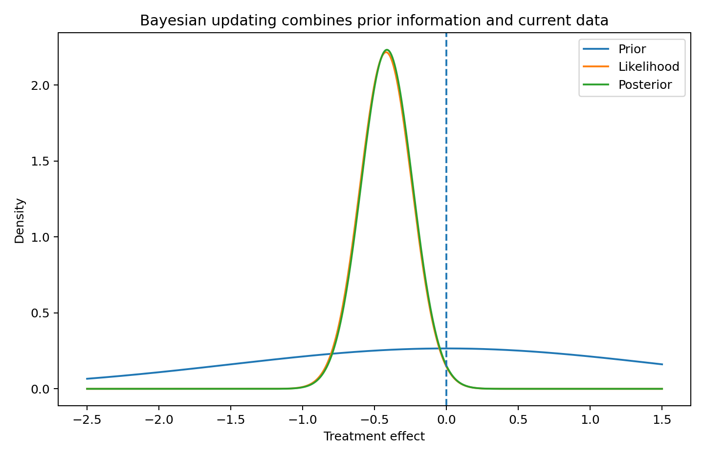
Posterior mean ≈ -0.414
Posterior SD ≈ 0.179
Posterior probability of benefit is approximately 0.99.

Visualising Bayesian updating

Credible intervals

A 95% credible interval means:

Under the model and prior, the posterior probability that the parameter lies in the interval is 95%.

This differs from the repeated-sampling interpretation of a confidence interval.

Prior choices

Priors can be:

• sceptical;
• enthusiastic;
• weakly informative;
• evidence based;
• hierarchical.

Avoid describing a very wide prior as automatically objective.

Prior predictive checks examine whether the prior implies plausible data.

Posterior predictive checks

Posterior predictive simulation compares observed data with data generated from the fitted model.

Systematic discrepancy signals model inadequacy.

Convergence diagnostics alone do not establish fit.

Interpreting the output

Presenting the analysis

Suggested reporting

Report prior rationale, likelihood, computational method, convergence, posterior predictive checks, sensitivity and decision thresholds [1], [2].

Applied Bayesian modelling texts and Stan-based computation provide broader guidance for prior specification, simulation and model checking [3], [4].

Common mistakes

Knowledge check

What combines with the likelihood?

Answer and reasoning

The prior distribution.

What does a 95% credible interval mean?

Answer and reasoning

A 95% posterior probability for the parameter under the model and prior.

Why perform prior sensitivity?

Answer and reasoning

Posterior conclusions can depend on prior assumptions, especially with limited data.

What is posterior predictive checking?

Answer and reasoning

Comparing observed data with replicated data generated from the posterior model.

Does Bayesian analysis remove design bias?

Answer and reasoning

No.

Key take-home messages

References

1. Spiegelhalter DJ, Abrams KR, Myles JP. Bayesian approaches to clinical trials and health-care evaluation. Chichester: Wiley; 2004.
2. Gelman A, Carlin JB, Stern HS, Dunson DB, Vehtari A, Rubin DB. Bayesian data analysis. 3rd ed. Boca Raton: CRC Press; 2013.
3. Kruschke JK. Doing Bayesian data analysis. 2nd ed. Boston: Academic Press; 2015.
4. Stan Development Team. RStan: the R interface to Stan. https://mc-stan.org/