Estimating One Proportion or Prevalence

Overview

A proportion is the fraction of observations in a defined denominator that meet a specified condition.

When the condition represents existing disease or another current state in a population at a defined time or period, the proportion is commonly described as prevalence.

Examples include:

• prevalence of uncontrolled hypertension among eligible clinic attendees;
• proportion of participants experiencing an adverse event;
• proportion of specimens with adequate quality;
• vaccination coverage among a defined population;
• proportion achieving treatment response.

A complete estimate requires:

• a clearly defined numerator;
• an appropriate denominator;
• the observed proportion or percentage;
• a confidence interval;
• and a description of the population, time frame and sampling process.

The interval method matters. The simple Wald interval can have poor coverage, especially when the sample is small or the proportion is near 0 or 1. Wilson’s score interval is a well-established alternative with better performance in many common settings [1], [2].

Why this matters

A statement such as:

Prevalence was 70%.

is incomplete.

The reader still needs to know:

• 70% of whom;
• during which period;
• how the condition was defined;
• how many participants were assessed;
• how many had missing status;
• whether the sample was representative;
• and how precise the estimate was.

A narrow confidence interval does not correct selection bias or misclassification. Statistical precision and epidemiological validity must be assessed separately.

When to use this method

Estimate one proportion when:

• the outcome has two mutually exclusive states;
• each independent analytical unit contributes one known status;
• the numerator is contained within the denominator;
• the target population and time frame are defined;
• and the objective is estimation rather than comparison.

A multi-category variable can also be summarised using a proportion for each category, but the category proportions are jointly constrained to sum to one.

Do not use a simple binomial interval unchanged when:

• observations are clustered;
• survey weights are required;
• repeated outcomes come from the same person;
• the denominator is person-time;
• or verification of outcome status depends on the observed result.

Research question and variables

The binary outcome is:

• uncontrolled = 1: meets the study definition;
• uncontrolled = 0: does not meet the definition.

The population parameter is:

$$p = P(\text{uncontrolled blood pressure})$$

The sample estimate is:

$$\hat{p} = \frac{x}{n}$$

where:

• $x$ is the number meeting the definition;
• $n$ is the number with known eligible status.

The objective is estimation. A test against 50% or another arbitrary value is unnecessary.

Data structure

Binary participant-level structure

simulated data

Table 1. First six participant records

participant_id	uncontrolled
H001	1
H002	0
H003	1
H004	1
H005	0
H006	1

Note: The complete simulated dataset contains 120 participants, of whom 84 meet the study definition.

Values should be labelled clearly. A code of 9 for missing status must not be analysed as a third disease category.

Statistical assumptions

Independence

The simple interval treats participant outcomes as independent.

If 120 observations come from 12 households, clinics or repeated visits, the effective information may be less than that supplied by 120 independent participants.

Missing status

The denominator should usually be the number with known status for a complete-record estimate. However, excluding missing status may bias prevalence if missingness is related to the condition.

Report:

• total eligible;
• assessed;
• missing or indeterminate;
• included in the denominator.

Misclassification

If the case definition has imperfect sensitivity or specificity, the observed proportion estimates apparent prevalence, not necessarily true prevalence.

A confidence interval quantifies sampling uncertainty under the classification rule. It does not correct measurement error.

How the method works

The sample proportion is:

For $x=84$ and $n=120$:

$$\hat{p} = \frac{84}{120} = 0.70$$

or 70.0%.

Wilson confidence interval

Let $z=z_{1-\alpha/2}$. The Wilson interval centre and half-width are:

Unlike the Wald interval, the Wilson interval remains within 0 and 1 and generally has more reliable coverage [1], [2].

Worked example

Reproducible R analysis

The following base-R function calculates the Wilson interval directly. This avoids generating an irrelevant hypothesis test when the objective is estimation.

wilson_ci <- function(x, n, conf.level = 0.95) {

  alpha <- 1 - conf.level
  z <- qnorm(1 - alpha / 2)
  p_hat <- x / n
  denominator <- 1 + z^2 / n

  centre <- (p_hat + z^2 / (2 * n)) / denominator
  half_width <- (
    z / denominator
  ) * sqrt(
    p_hat * (1 - p_hat) / n +
      z^2 / (4 * n^2)
  )

  c(
    estimate = p_hat,
    lower = centre - half_width,
    upper = centre + half_width
  )
}

result <- wilson_ci(x = 84, n = 120)

output <- data.frame(
  numerator = 84,
  denominator = 120,
  prevalence_percent = round(100 * result["estimate"], 1),
  ci_lower_percent = round(100 * result["lower"], 1),
  ci_upper_percent = round(100 * result["upper"], 1)
)

print(output, row.names = FALSE)

Cleaned R output

 numerator denominator prevalence_percent ci_lower_percent ci_upper_percent
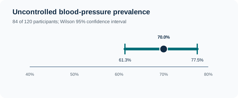
        84         120               70.0             61.3             77.5

Base R also provides binom.test() for an exact Clopper–Pearson interval and prop.test() for score-based large-sample procedures [3]. The method used should be stated because different valid intervals have different coverage and width.

Interpreting the output

Presenting the results

Table 2. Estimated prevalence of uncontrolled blood pressure

Note: The interval is the two-sided Wilson score interval. All data are simulated.

Suggested reporting

Exact, score and design-based intervals MMed extension

The Clopper–Pearson interval controls coverage conservatively through the binomial distribution but can be wider than necessary.

Wilson and related score intervals often provide a useful balance between coverage and width for an independent binomial sample [1], [2].

Complex surveys require design-based intervals that incorporate weights, strata and clusters. A binomial interval applied to an unweighted count does not represent a complex sampling design.

Common mistakes

Knowledge check

What is the numerator in the worked example?

Answer and reasoning

The numerator is the 84 participants who meet the prespecified uncontrolled blood-pressure definition.

Why must missing outcome status not be coded as zero?

Answer and reasoning

Zero represents a known outcome-negative participant. Missing status is unknown and must be handled and reported separately; recoding it as zero biases the proportion downward.

What does the Wilson 95% CI of 61.3% to 77.5% describe?

Answer and reasoning

It describes sampling uncertainty for the population prevalence under the stated design and interval procedure. It does not quantify selection or measurement bias.

Is 70 cases per 1,000 person-years a prevalence?

Answer and reasoning

No. That denominator represents person-time, so the measure is an incidence rate rather than a proportion or prevalence.

Why may a simple Wilson interval be inappropriate for a cluster sample?

Answer and reasoning

Participants within clusters may be correlated, so the simple binomial variance understates uncertainty. The design and clustering must be incorporated.

Key take-home messages

References

1. Wilson EB. Probable inference, the law of succession, and statistical inference. J Am Stat Assoc. 1927;22(158):209–212. https://doi.org/10.1080/01621459.1927.10502953
2. Brown LD, Cai TT, DasGupta A. Interval estimation for a binomial proportion. Stat Sci. 2001;16(2):101–133. https://doi.org/10.1214/ss/1009213286
3. R Core Team. Exact binomial test and test of equal or given proportions. R documentation, package stats version 4.6.1. Vienna: R Foundation for Statistical Computing; 2026. https://stat.ethz.ch/R-manual/R-devel/library/stats/html/prop.test.html
4. R Core Team. R: a language and environment for statistical computing. Version 4.6.1. Vienna: R Foundation for Statistical Computing; 2026. https://www.R-project.org/