
Part 7 · Module 6
Stratified Analysis
Learn how to examine stratum-specific categorical associations and estimate a Mantel-Haenszel common odds ratio using reproducible R output.
Learning outcomes
After completing this lecture, you should be able to:
- Construct and interpret stratum-specific two-by-two tables.
- Distinguish confounding from effect modification conceptually.
- Calculate stratum-specific odds ratios and a Mantel-Haenszel common odds ratio.
- Interpret the Cochran-Mantel-Haenszel test and confidence interval.
- Explain why a common effect should not conceal important heterogeneity.
- Use reproducible R code to perform a stratified categorical analysis.
Overview
Stratified analysis divides data into clinically meaningful levels of a third variable and examines the exposure–outcome association within each stratum.
It can help researchers:
- describe confounding;
- identify effect modification;
- control a categorical stratification variable;
- assess whether a crude association is consistent across subgroups;
- estimate a common odds ratio when a common effect is scientifically reasonable.
The Mantel–Haenszel method combines information from several two-by-two tables while controlling for the stratification variable [1].
A common estimate should not be reported until the stratum-specific associations have been examined.
Why this matters
A crude two-by-two table can combine groups with different:
- baseline risks;
- exposure prevalence;
- age distribution;
- disease severity;
- clinical settings.
The resulting association may differ from the within-stratum associations.
However, not every difference between crude and adjusted estimates is confounding, and not every variation among strata is meaningful effect modification.
Confounding is a causal-structure problem and should be assessed using epidemiological knowledge rather than a crude statistical rule [4]. Effect modification describes genuine variation in the selected effect measure across levels of another variable.
When to use this method
Use stratified analysis when:
- exposure and outcome are categorical;
- a small number of clinically meaningful strata are defined;
- each participant belongs to one stratum;
- two-by-two tables can be formed within strata;
- and a crude association may be distorted or modified by the stratifying variable.
Regression is usually preferable when:
- many confounders are present;
- variables are continuous;
- interactions require flexible modelling;
- or standardised risks rather than odds ratios are the target.
Research question and variables
The binary variables are:
- exposure: exposed or unexposed;
- outcome: adverse outcome or no adverse outcome.
The stratification variable is age group.
Within each stratum , the table is:
| Outcome | No outcome | |
|---|---|---|
| Exposed | ||
| Unexposed |
The stratum-specific odds ratio is:
Data structure
Age-stratified two-by-two tables
simulated dataTable 1. Adverse outcome by exposure and age stratum
| Age stratum | Exposed outcome / total | Unexposed outcome / total | Stratum OR |
|---|---|---|---|
| Younger | 20 / 100 | 10 / 100 | 2.25 |
| Middle-aged | 30 / 100 | 20 / 100 | 1.71 |
| Older | 25 / 100 | 20 / 100 | 1.33 |
Note: OR = odds ratio. All counts are simulated.
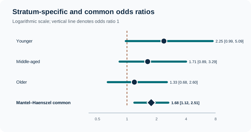
The stratum-specific estimates decline across age, but their intervals are wide. Statistical and clinical heterogeneity should both be considered.
Statistical assumptions
Very broad age strata can leave residual confounding. Very narrow strata can create sparse tables.
How the method works
The Mantel–Haenszel common odds ratio is:
The Cochran–Mantel–Haenszel test assesses conditional association while controlling for strata under a common-association framework [1], [2].
Worked example
Reproducible R analysis
Base R implements the Cochran–Mantel–Haenszel procedure using mantelhaen.test() [3].
younger <- matrix(
  c(20, 80, 10, 90),
  nrow = 2,
  byrow = TRUE
)

middle <- matrix(
  c(30, 70, 20, 80),
  nrow = 2,
  byrow = TRUE
)

older <- matrix(
  c(25, 75, 20, 80),
  nrow = 2,
  byrow = TRUE
)

strata <- array(
  c(younger, middle, older),
  dim = c(2, 2, 3),
  dimnames = list(
    Exposure = c("Exposed", "Unexposed"),
    Outcome = c("Outcome", "No outcome"),
    Age = c("Younger", "Middle-aged", "Older")
  )
)

mh_fit <- mantelhaen.test(
  strata,
  correct = FALSE,
  conf.level = 0.95
)

stratum_or <- apply(
  strata,
  3,
  function(tab) {
    (tab[1, 1] * tab[2, 2]) /
      (tab[1, 2] * tab[2, 1])
  }
)

mh_fit
stratum_or

output <- data.frame(
  mh_chi_square = unname(mh_fit$statistic),
  df = unname(mh_fit$parameter),
  p_value = mh_fit$p.value,
  common_odds_ratio = unname(mh_fit$estimate),
  ci_lower = mh_fit$conf.int[1],
  ci_upper = mh_fit$conf.int[2]
)

round(output, 3)
R output
	Mantel-Haenszel chi-squared test without continuity correction

Mantel-Haenszel X-squared = 6.3538, df = 1, p-value = 0.01171
alternative hypothesis: true common odds ratio is not equal to 1
95 percent confidence interval:
 1.119946 2.507166
sample estimates:
common odds ratio
         1.675676
Interpreting the output
Presenting the results
Table 2. Stratum-specific and common odds ratios
| Estimate | Odds ratio | 95% CI |
|---|---|---|
| Younger | 2.25 | 0.99 to 5.09 |
| Middle-aged | 1.71 | 0.89 to 3.29 |
| Older | 1.33 | 0.68 to 2.60 |
| Mantel–Haenszel common | 1.68 | 1.12 to 2.51 |
Cochran–Mantel–Haenszel , .
Suggested reporting
Confounding versus effect modification MMed extension
A variable may act as:
- a confounder on one causal structure;
- an effect modifier on a chosen effect scale;
- both;
- neither.
Confounding is not defined merely by statistical association with exposure and outcome.
Effect modification depends on the scale. Effects can be homogeneous on the risk-ratio scale but heterogeneous on the risk-difference scale.
Regression interaction terms provide a more flexible framework but still require prespecified effect scales and careful interpretation.
Common mistakes
Knowledge check
Why examine stratum-specific odds ratios before the common estimate?
Answer and reasoning
A common estimate can conceal important variation. The stratum-specific results reveal whether one summary is clinically and statistically defensible.
What does the Mantel-Haenszel odds ratio control for?
Answer and reasoning
It combines within-stratum information, thereby controlling for the categorical stratification variable under the method’s assumptions.
Does a common odds ratio of 1.68 mean risk is 68% higher?
Answer and reasoning
No. It means the conditional odds are estimated to be 1.68 times as high. Odds and risks are different quantities.
Can overlapping stratum-specific confidence intervals prove no effect modification?
Answer and reasoning
No. Overlap is not a formal or sufficiently sensitive test, and clinically important variation may remain.
When should regression replace stratification?
Answer and reasoning
When many covariates, continuous adjustment, interactions, sparse strata or adjusted risks on other effect scales are required.
Key take-home messages
References
- Mantel N, Haenszel W. Statistical aspects of the analysis of data from retrospective studies of disease. J Natl Cancer Inst. 1959;22(4):719–748.
- Cochran WG. Some methods for strengthening the common chi-square tests. Biometrics. 1954;10(4):417–451. https://doi.org/10.2307/3001616
- R Core Team. Cochran-Mantel-Haenszel chi-squared test for count data. R documentation, package stats version 4.6.1. Vienna: R Foundation for Statistical Computing; 2026. https://stat.ethz.ch/R-manual/R-devel/library/stats/html/mantelhaen.test.html
- Lash TL, VanderWeele TJ, Haneuse S, Rothman KJ. Modern epidemiology. 4th ed. Philadelphia: Wolters Kluwer; 2021.
These notes support learning and research planning and do not replace statistical consultation for a specific study.