Prediction Models in Medicine

Overview

A clinical prediction model estimates an individual’s probability or expected value of a current or future outcome.

Examples include predicting:

• in-hospital mortality;
• treatment response;
• disease recurrence;
• diagnostic probability;
• complications.

Prediction differs from causal inference. A predictor can be useful without causing the outcome, and a causal factor may add little predictive information.

Why this matters

A model can appear accurate in its development data and fail in new patients because of overfitting, population differences or measurement inconsistency.

Performance should be evaluated using:

• calibration;
• discrimination;
• overall prediction error;
• clinical utility;
• external validation.

TRIPOD+AI provides current reporting guidance for regression and machine-learning prediction models [1]. PROBAST+AI assesses quality, risk of bias and applicability [2].

When to use this method

Develop a prediction model only when:

• the target population and clinical use are clear;
• outcome, time horizon and predictor timing are defined;
• predictors will be available at intended use;
• sample size supports candidate complexity;
• internal validation is planned;
• external validation is feasible.

Research question and variables

The target is the probability of controlled follow-up blood pressure.

Candidate predictors are available before the prediction time.

The model output is:

$$\hat{p}_i=P(Y_i=1\mid\mathbf{X}_i)$$

Data structure

Development and validation roles

simulated data

Dataset	Participants	Purpose
Development	120	Estimate model coefficients
Validation	60	Evaluate performance without refitting

A truly external validation dataset should differ in place, time, setting or investigators in a clinically relevant way.

Statistical assumptions

How the method works

Discrimination

For a binary outcome, the area under the receiver operating characteristic curve, also called the c-statistic, is the probability that a randomly selected participant with the outcome receives a higher predicted risk than one without it.

Calibration

Calibration compares predicted with observed probabilities.

Important summaries include:

• calibration-in-the-large or intercept;
• calibration slope;
• calibration plot.

An ideal validation intercept is 0 and slope is 1.

Brier score

Define the intended use

A prediction model should specify:

• who will be assessed;
• where and when it will be used;
• which outcome and time horizon are predicted;
• what decision the prediction may support;
• which predictors are available at that moment.

A model for prognosis after hospital admission is not automatically suitable for community screening because the populations, measurements and baseline risks differ.

Predictor timing and data leakage

Predictors must be available at the intended prediction time. Including information obtained after outcome onset or after a treatment decision creates leakage and exaggerates performance.

Preprocessing steps can also leak information. Imputation models, variable transformations and feature selection should be estimated within each resampling or development set rather than using the complete dataset before validation.

Sample size and candidate parameters

Prediction-model sample size should be based on the outcome proportion, number of candidate parameters, anticipated model fit and desired precision of predictions and performance measures.

Nonlinear terms, categorical indicators and interactions all consume parameters. A large total sample can still be inadequate when the outcome is rare or the model is highly complex.

Internal validation and optimism

Internal validation estimates how much apparent performance is inflated because the model was tailored to the development sample.

Bootstrap validation is often efficient:

1. sample participants with replacement;
2. repeat the entire modelling process;
3. evaluate the model in the bootstrap and original samples;
4. estimate optimism;
5. average optimism across repetitions.

Cross-validation can also estimate out-of-sample performance, particularly for tuning. Neither method replaces evaluation in a genuinely external population.

Calibration

Calibration-in-the-large compares the average predicted risk with the observed event rate. A negative calibration intercept generally indicates overprediction when the slope is fixed at one.

The calibration slope assesses prediction extremity. A slope below one indicates that high risks are too high and low risks too low. A slope above one indicates predictions that are not extreme enough.

A smooth calibration plot is more informative than dividing predictions into arbitrary groups.

Discrimination

The c-statistic measures ranking, not probability accuracy. It can remain unchanged when every predicted risk is systematically doubled, even though calibration becomes poor.

For time-to-event outcomes, discrimination must accommodate censoring and a defined time horizon. For multicategory outcomes, several discrimination summaries may be required.

Overall performance

The Brier score combines calibration and discrimination through squared probability error. It should be compared with a null or benchmark model because its attainable range depends on outcome prevalence.

The logarithmic score is another proper scoring rule that penalises confident incorrect predictions strongly.

Clinical utility

Decision-curve analysis evaluates net benefit across plausible risk thresholds. It compares model-guided decisions with strategies such as treating everyone or no one.

A high AUC does not guarantee positive net benefit. Thresholds should reflect clinical consequences, available interventions and patient preferences.

External validation

External validation applies the fixed model—without re-estimating coefficients—to new data. Validation can be temporal, geographic, setting-based or investigator-independent.

Report differences in eligibility, predictor measurement, outcome definition, missingness and treatment pathways. Poor calibration may reflect changed baseline risk rather than useless predictor effects.

Model updating

A model with preserved discrimination but shifted baseline risk may need intercept recalibration. More extensive updating may adjust the calibration slope or re-estimate selected coefficients.

Updating should be evaluated in separate data. Repeatedly modifying and evaluating a model in the same validation dataset converts it into a new development exercise.

Fairness and subgroup performance

Overall performance can conceal poor calibration or discrimination in clinically important groups. Evaluate performance across prespecified demographic and clinical subgroups while recognising uncertainty and multiplicity.

Fairness assessment should consider measurement quality, access to care, consequences of errors and whether subgroup differences reflect structural inequities.

Reproducibility and implementation

A deployable model requires the full equation or code, predictor definitions, units, handling of missing values and calculation sequence.

Implementation should include monitoring for data drift, calibration change and unintended clinical consequences. Publication of a model is the beginning of evaluation rather than the end.

Worked example

Reproducible R analysis

make_hypertension_data <- function(n = 180) {
  set.seed(4583)
  i <- seq_len(n)

  data <- data.frame(
    participant_id = sprintf("H%03d", i),
    age = round(runif(n, 30, 80)),
    male = rbinom(n, 1, 0.5),
    bmi = pmin(pmax(round(rnorm(n, 27, 3.5), 1), 18), 40),
    physical_activity = round(runif(n, 2, 7), 1),
    telemonitoring = rbinom(n, 1, 0.5)
  )

  data$adherence <- 4 + runif(n, 0, 5) -
    0.015 * (data$age - 55) + 0.4 * data$telemonitoring
  data$baseline_sbp <- 92 + 0.52 * data$age + 0.85 * data$bmi +
    2.8 * data$male - 1.3 * data$physical_activity + rnorm(n, 0, 4)
  data$followup_sbp <- 58 + 0.47 * data$baseline_sbp +
    0.10 * data$age + 0.52 * data$bmi - 2.0 * data$adherence +
    2.0 * data$male - 4.5 * data$telemonitoring -
    0.55 * data$telemonitoring * (data$bmi - 27) +
    0.006 * (data$age - 55)^2 + rnorm(n, 0, 5)

  data
}

hypertension <- make_hypertension_data()

hypertension$controlled <- as.integer(
  hypertension$followup_sbp < 130
)

development <- hypertension[1:120, ]
validation <- hypertension[121:180, ]

fit <- glm(
  controlled ~ telemonitoring + baseline_sbp +
    age + bmi + adherence + male,
  data = development,
  family = binomial(link = "logit")
)

validation$predicted_probability <- predict(
  fit,
  newdata = validation,
  type = "response"
)

auc_rank <- function(outcome, probability) {
  ranks <- rank(probability)
  n1 <- sum(outcome == 1)
  n0 <- sum(outcome == 0)

  (
    sum(ranks[outcome == 1]) -
      n1 * (n1 + 1) / 2
  ) / (n1 * n0)
}

c_statistic <- auc_rank(
  validation$controlled,
  validation$predicted_probability
)

brier_score <- mean(
  (
    validation$controlled -
      validation$predicted_probability
  )^2
)

linear_predictor <- qlogis(
  validation$predicted_probability
)

calibration_model <- glm(
  controlled ~ linear_predictor,
  data = validation,
  family = binomial(link = "logit")
)

output <- data.frame(
  observed_rate = mean(validation$controlled),
  mean_prediction = mean(validation$predicted_probability),
  c_statistic = c_statistic,
  brier_score = brier_score,
  calibration_intercept = coef(calibration_model)[1],
  calibration_slope = coef(calibration_model)[2]
)

round(output, 3)

Cleaned R output

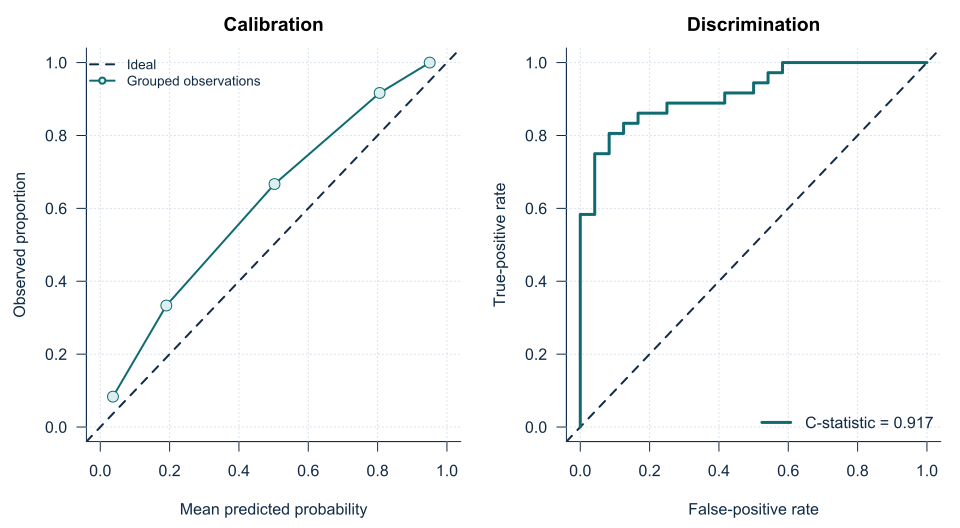
Validation measure          Estimate
Observed outcome rate         0.600
Mean predicted probability    0.497
C-statistic                    0.917
Brier score                    0.125
Calibration intercept          0.919
Calibration slope              1.127

Interpreting the output

Presenting the results

Present discrimination, calibration, overall prediction error and clinical utility rather than one performance statistic alone.

Visualising validation performance

Suggested reporting

Why a random train–test split is often inefficient MMed extension

A single split discards information from model development and gives unstable validation estimates.

Bootstrap validation or repeated cross-validation generally uses data more efficiently for internal validation. Independent external data remain necessary for transportability assessment [3], [4], with the validation design and reporting described explicitly [5].

Common mistakes

Knowledge check

What does the c-statistic measure?

Answer and reasoning

It measures ranking discrimination: the probability that a participant with the outcome receives a higher prediction than one without it.

What does a calibration slope below one suggest?

Answer and reasoning

Predictions are generally too extreme, often because of overfitting or differences between development and validation settings.

Why is AUC alone insufficient?

Answer and reasoning

A model can discriminate well while probabilities are systematically wrong or clinically unhelpful.

Why is a single split inefficient?

Answer and reasoning

It reduces development information and produces an imprecise validation assessment, especially in small datasets.

What distinguishes external validation?

Answer and reasoning

The model is evaluated without refitting in a meaningfully independent population, setting, place or time.

Key take-home messages

References

1. Collins GS, Moons KGM, Dhiman P, Riley RD, Beam AL, Van Calster B, et al. TRIPOD+AI statement: updated guidance for reporting clinical prediction models that use regression or machine learning methods. BMJ. 2024;385:e078378. https://doi.org/10.1136/bmj-2023-078378
2. Moons KGM, Damen JAA, Kaul T, et al. PROBAST+AI: an updated quality, risk of bias, and applicability assessment tool for prediction models using regression or artificial intelligence methods. BMJ. 2025;388:e082505. https://doi.org/10.1136/bmj-2024-082505
3. Riley RD, Ensor J, Snell KIE, Harrell FE Jr, Martin GP, Reitsma JB, et al. Calculating the sample size required for developing a clinical prediction model. BMJ. 2020;368:m441. https://doi.org/10.1136/bmj.m441
4. Steyerberg EW. Clinical prediction models. 2nd ed. Cham: Springer; 2019. https://doi.org/10.1007/978-3-030-16399-0
5. Riley RD, Archer L, Snell KIE, Ensor J, Dhiman P, Martin GP, et al. Evaluation of clinical prediction models (part 2): how to undertake an external validation study. BMJ. 2024;384:e074820. https://doi.org/10.1136/bmj-2023-074820