Generalised Estimating Equations

Overview

Generalised estimating equations, abbreviated GEE, extend generalised linear models to correlated observations.

GEE separates the marginal mean model, working correlation and sandwich variance.

The coefficients have a population-averaged interpretation. The method was introduced for longitudinal generalised linear models by Liang and Zeger [1].

Why this matters

A conventional linear or logistic model assumes independent observations. GEE allows repeated or clustered outcomes while retaining familiar mean structures and link functions.

GEE is useful when the scientific target is the average population response rather than participant-specific random effects.

When to use this method

Use GEE when observations are correlated within identifiable clusters, clusters are independent, a population-averaged effect is the target and the cluster count supports sandwich inference.

Research question and variables

Data structure

Required GEE variables

simulated data

Table 1. GEE data elements

Variable	Purpose
id	Cluster identifier
month	Ordered repeated time
group	Treatment group
sbp	Numerical outcome
age, male	Baseline covariates
Row order	Sorted by participant and time

The data should be sorted so observations from one participant occur together.

Statistical assumptions

Working correlation structures

• Independence: zero working correlation.
• Exchangeable: one common within-cluster correlation.
• Autoregressive: correlation decreases with time separation.
• Unstructured: one correlation for every visit pair.

The working correlation supports efficiency but is not usually the main scientific target.

How the method works

The sandwich variance uses empirical cluster residual contributions. It is robust to working-correlation misspecification when the mean model is correct and the cluster count is sufficiently large.

Worked example

Worked analysis in R

make_longitudinal_data <- function(n = 120) {
  records <- vector("list", n * 3)
  row_number <- 1

  for (participant_id in seq_len(n)) {
    group <- as.integer(participant_id %% 2 == 0)
    age <- 35 + ((7 * participant_id) %% 41)
    male <- as.integer(participant_id %% 3 == 0)

    random_intercept <-
      7 * sin(participant_id * 0.71) +
      3 * cos(participant_id * 0.19)

    random_slope <-
      0.45 * sin(participant_id * 0.37)

    for (month in c(0, 3, 6)) {
      residual <-
        3.5 * sin(participant_id * 1.13 + month * 0.91) +
        1.2 * cos(participant_id * 0.23 + month * 0.33)

      sbp <-
        151 +
        0.18 * (age - 55) +
        1.8 * male +
        random_intercept -
        1.5 * month -
        0.4 * group -
        0.75 * group * month +
        random_slope * month +
        residual

      records[[row_number]] <- data.frame(
        id = participant_id,
        group = group,
        age = age,
        male = male,
        month = month,
        sbp = sbp
      )

      row_number <- row_number + 1
    }
  }

  longitudinal <- do.call(rbind, records)

  longitudinal$group <- factor(
    longitudinal$group,
    levels = c(0, 1),
    labels = c("Usual care", "Telemonitoring")
  )

  longitudinal <- longitudinal[
    order(longitudinal$id, longitudinal$month),
  ]

  rownames(longitudinal) <- NULL
  longitudinal
}

longitudinal <- make_longitudinal_data()

library(geepack)

gee_fit <- geeglm(
  sbp ~ group * month + age + male,
  id = id,
  data = longitudinal,
  family = gaussian(link = "identity"),
  corstr = "exchangeable",
  std.err = "san.se"
)

summary(gee_fit)

coefficient_table <- coef(summary(gee_fit))

output <- data.frame(
  term = rownames(coefficient_table),
  estimate = coefficient_table[, "Estimate"],
  robust_se = coefficient_table[, "Std.err"],
  wald = coefficient_table[, "Wald"],
  p_value = coefficient_table[, "Pr(>|W|)"]
)

output
gee_fit$geese$alpha

Selected analysis output

Term                         Estimate   Robust SE   95% CI
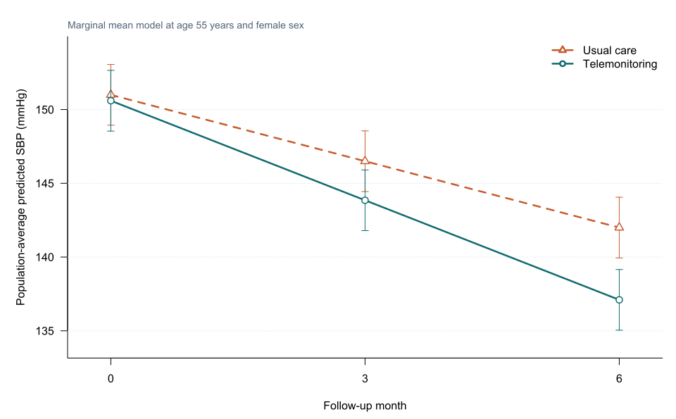
Telemonitoring at baseline    -0.542      1.015     -2.532 to 1.448
Month                         -1.519      0.066     -1.648 to -1.390
Telemonitoring × month        -0.737      0.093     -0.919 to -0.554
Age                            0.188      0.038      0.113 to 0.263
Male versus female             1.588      1.077     -0.523 to 3.700

Working correlation alpha = 0.736

Small numerical differences can occur across package versions and variance conventions.

Visualising marginal predictions

Missing outcomes

Ordinary GEE is not automatically valid for every missing-at-random process.

Possible approaches include inverse-probability-weighted GEE, multiple imputation followed by GEE and sensitivity analyses under alternative missingness assumptions.

Number of clusters

Sandwich variance is asymptotic in the number of independent clusters.

With few clusters, ordinary robust SEs can be biased downward. Small-sample corrections or alternative analyses may be required.

Interpreting the output

Presenting the results

Suggested reporting

Report family and link, cluster identifier, working correlation, variance estimator, cluster count, time scale, effect interpretation and missing-data method [1], [2], [3]. Broader covariance and missing-data considerations are developed by Diggle and colleagues [4].

Common mistakes

Knowledge check

What does a GEE coefficient usually describe?

Answer and reasoning

A population-averaged association on the selected link scale.

What is the purpose of the working correlation?

Answer and reasoning

It represents within-cluster dependence for efficiency; robust variance protects against some misspecification.

What does the interaction coefficient of −0.737 mean?

Answer and reasoning

The telemonitoring mean declines by an additional 0.737 mmHg per month compared with usual care.

Why can ordinary GEE be problematic with ten clinics?

Answer and reasoning

Sandwich inference relies on many independent clusters, and ten may be too few.

Does alpha 0.736 mean every observed correlation equals 0.736?

Answer and reasoning

No. It is one fitted working-correlation summary.

Key take-home messages

References

1. Liang KY, Zeger SL. Longitudinal data analysis using generalized linear models. Biometrika. 1986;73(1):13–22. https://doi.org/10.1093/biomet/73.1.13
2. Højsgaard S, Halekoh U, Yan J. The R package geepack for generalized estimating equations. J Stat Softw. 2006;15(2):1–11. https://doi.org/10.18637/jss.v015.i02
3. Zeger SL, Liang KY, Albert PS. Models for longitudinal data: a generalized estimating equation approach. Biometrics. 1988;44(4):1049–1060. https://doi.org/10.2307/2531734
4. Diggle PJ, Heagerty P, Liang KY, Zeger SL. Analysis of longitudinal data. 2nd ed. Oxford: Oxford University Press; 2002. https://doi.org/10.1093/oso/9780198524847.001.0001