One-Sample t-Test

Overview

A one-sample t-test compares the mean of one population with a prespecified reference value.

Examples include testing whether:

• mean systolic blood pressure differs from a service benchmark;
• mean laboratory recovery differs from 100%;
• mean change from baseline differs from zero;
• mean device bias differs from zero; or
• mean patient-reported score differs from an established reference mean.

The test is appropriate only when the reference value is scientifically meaningful and specified independently of the observed sample.

The analysis should not be reported as a p-value alone. The estimated mean difference and 95% confidence interval show the direction, magnitude and precision of the comparison.

Why this matters

Suppose a sample mean is 136.4 mmHg and the prespecified reference mean is 140 mmHg.

The one-sample t-test asks:

If the population mean were exactly 140 mmHg, how unusual would an estimated mean this far from 140 be relative to its standard error?

It does not ask:

• whether every participant differs from 140 mmHg;
• whether 140 mmHg is an individual diagnostic threshold;
• whether the null hypothesis has a particular probability;
• or whether the observed difference is clinically important.

The t distribution was developed to account for uncertainty introduced when the population standard deviation is unknown and estimated from the same sample [1].

When to use this method

Use a one-sample t-test when:

• one numerical outcome is observed;
• one independent sample is available;
• the arithmetic population mean is the estimand;
• the population standard deviation is unknown;
• a scientifically justified reference mean is prespecified;
• and the assumptions of the t-based procedure are sufficiently reasonable.

Do not use it to compare:

• a sample mean with its own rounded or historical value selected after looking at the data;
• two independent groups;
• paired values without first defining the paired difference;
• an ordinal outcome mean without justification;
• a proportion;
• or several repeated measurements treated as independent.

A one-sample test of mean change can be appropriate if one change score is calculated for each independent participant. It is then mathematically equivalent to a paired t-test on the original before-and-after values.

Research question and variables

The population parameter is:

$$\mu = \text{population mean systolic blood pressure}$$

The null reference is:

$$\mu_0=140\text{ mmHg}$$

The two-sided hypotheses are:

$$H_0:\mu=140\text{ mmHg}$$ $$H_1:\mu\ne140\text{ mmHg}$$

The estimated effect is the mean difference from the reference:

$$\bar{x}-\mu_0$$

The contrast direction in this lecture is:

clinic population mean minus 140 mmHg.

A negative difference indicates a mean below the reference.

Data structure

The analytical dataset contains one row per participant.

Structure for a one-sample t-test

simulated data

Table 1. Example records

participant_id	sbp_mmHg
H001	135
H002	129
H003	144
H004	142
H005	142
H006	143

Note: The complete simulated dataset contains 40 participants. The reference value of 140 mmHg is not stored as a second group.

Creating 40 duplicate rows containing the reference value would be incorrect. The benchmark is a fixed hypothesised mean, not another sample with sampling variability.

Statistical assumptions

Normality and robustness

For a small sample, the exact one-sample t-test assumes observations arise from a normal population.

The test can be reasonably robust to moderate departures as sample size increases, but heavy tails, severe skewness and influential observations may affect its type I error, power and confidence-interval coverage [2].

Do not choose or reject the method solely using a Shapiro–Wilk p-value. Inspect:

• a dot plot or histogram;
• a quantile–quantile plot;
• data-quality records;
• clinically unusual values;
• and the influence of plausible observations.

Independence

Independence concerns the analytical units, not the software rows.

Multiple readings from one participant require either:

• one prespecified participant-level summary; or
• a repeated-measurement model.

Meaning of the reference

The test may be mathematically valid but scientifically unhelpful if the reference mean has no decision relevance.

A clinical threshold for an individual is not automatically an appropriate population-mean null value.

How the method works

The one-sample t statistic is:

The statistic expresses the estimated difference in standard-error units.

A large absolute value indicates that the observed mean is far from the reference relative to sampling variability.

For a two-sided test, evidence in either direction contributes to the p-value.

Worked example

Reproducible R analysis

Base R performs the test using t.test(). The official function accepts the numeric vector, hypothesised mean, alternative and confidence level and returns the statistic, degrees of freedom, p-value, confidence interval and sample estimate [3].

bp <- data.frame(
  participant_id = sprintf("H%03d", 1:40),
  sbp_mmHg = c(
    135, 129, 144, 142, 142, 143, 126, 126, 125, 120,
    152, 144, 132, 140, 141, 132, 131, 125, 145, 133,
    118, 145, 154, 128, 120, 153, 144, 144, 142, 141,
    133, 120, 152, 124, 151, 126, 145, 126, 122, 159
  )
)

fit <- t.test(
  bp$sbp_mmHg,
  mu = 140,
  alternative = "two.sided",
  conf.level = 0.95
)

fit

R console output

	One Sample t-test

data:  bp$sbp_mmHg
t = -2.0681, df = 39, p-value = 0.04531
alternative hypothesis: true mean is not equal to 140
95 percent confidence interval:
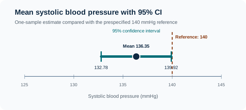
 132.7802 139.9198
sample estimates:
mean of x
   136.35

The confidence interval printed by t.test() is for the population mean. The following code produces a clean table and the interval for the mean difference from 140 mmHg.

difference_ci <- fit$conf.int - 140

result <- data.frame(
  observed_n = sum(!is.na(bp$sbp_mmHg)),
  mean_mmHg = round(unname(fit$estimate), 2),
  reference_mmHg = 140,
  mean_difference_mmHg = round(unname(fit$estimate) - 140, 2),
  t = round(unname(fit$statistic), 3),
  df = unname(fit$parameter),
  p_value = round(fit$p.value, 3),
  difference_ci_lower = round(difference_ci[1], 2),
  difference_ci_upper = round(difference_ci[2], 2)
)

print(result, row.names = FALSE)

# Reproducibility checks

Cleaned R output

 observed_n mean_mmHg reference_mmHg mean_difference_mmHg      t df p_value difference_ci_lower difference_ci_upper
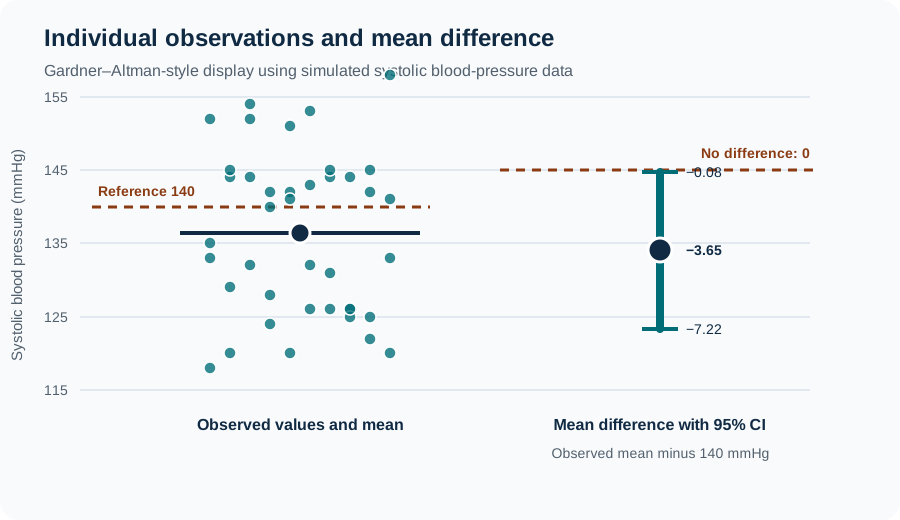
         40    136.35            140                -3.65 -2.068 39   0.045               -7.22               -0.08

The explicit dataset and validation checks allow readers to reproduce the analysis and independently verify every displayed value.

Interpreting the output

Why the interval and p-value agree

The two-sided 95% CI for the population mean is 132.78 to 139.92 mmHg and excludes 140 mmHg narrowly.

The corresponding two-sided test therefore gives $p<0.05$ when the same t-based method is used.

The interval provides more information because it shows the magnitude and precision of the difference [5].

Presenting the results

Table 2. One-sample comparison with the 140 mmHg reference mean

Note: The contrast is the clinic population mean minus 140 mmHg. Negative values indicate a lower mean. All values are simulated.

Visualising the estimate

Avoid presenting only:

The result was statistically significant.

That wording omits the outcome level, contrast, magnitude and uncertainty.

Suggested reporting

Alternatives when the t-based procedure is unsuitable MMed extension

Possible alternatives depend on the estimand.

• A bootstrap interval can target the mean under a suitable resampling design.
• A permutation or randomisation procedure may test a sharp null under an exchangeability framework.
• A one-sample Wilcoxon signed-rank test targets a rank-based symmetry-related contrast, not automatically the population mean.
• A sign test concerns the probability of observations lying above or below a reference and is related to a median under continuity assumptions.
• A model for transformed positive data may estimate a geometric mean or ratio rather than an arithmetic mean.

The alternative should be selected because it matches the scientific target and data structure, not because it produces a preferred p-value.

Common mistakes

Knowledge check

What is the null hypothesis in the worked example?

Answer and reasoning

The population mean systolic blood pressure among the defined clinic population equals 140 mmHg. The null concerns the population mean, not every participant’s value.

What does the t-statistic of −2.068 mean?

Answer and reasoning

The observed sample mean lies approximately 2.07 estimated standard errors below the reference mean. The negative sign indicates the direction of the contrast.

Why should the 140 mmHg reference not be entered as a second sample of 40 identical values?

Answer and reasoning

The benchmark is a fixed hypothesised mean, not a sampled group with its own variability. Creating an artificial group changes the statistical problem and produces an invalid variance structure.

Does p = 0.045 prove that the difference is clinically important?

Answer and reasoning

No. The p-value addresses compatibility with the exact null under the model. Clinical importance depends on the estimated difference, confidence interval, consequences, context and prespecified decision criteria.

What would p ≥ 0.05 mean in this test?

Answer and reasoning

It would mean that the null mean was not rejected at the selected significance level. It would not prove that the population mean equals 140 mmHg; the confidence interval would show which differences remain compatible.

Key take-home messages

References

1. Student. The probable error of a mean. Biometrika. 1908;6(1):1–25. https://doi.org/10.1093/biomet/6.1.1
2. Lumley T, Diehr P, Emerson S, Chen L. The importance of the normality assumption in large public health data sets. Annu Rev Public Health. 2002;23:151–169. https://doi.org/10.1146/annurev.publhealth.23.100901.140546
3. R Core Team. Student’s t-test. R documentation, package stats version 4.6.1. Vienna: R Foundation for Statistical Computing; 2026. https://search.r-project.org/R/refmans/stats/html/t.test.html
4. Greenland S, Senn SJ, Rothman KJ, Carlin JB, Poole C, Goodman SN, et al. Statistical tests, P values, confidence intervals, and power: a guide to misinterpretations. Eur J Epidemiol. 2016;31(4):337–350. https://doi.org/10.1007/s10654-016-0149-3
5. Gardner MJ, Altman DG. Confidence intervals rather than P values: estimation rather than hypothesis testing. Br Med J (Clin Res Ed). 1986;292(6522):746–750. https://doi.org/10.1136/bmj.292.6522.746