Poisson and Negative Binomial Regression

Overview

Count outcomes are non-negative integers such as:

• unscheduled visits;
• hospital admissions;
• falls;
• infections;
• adverse events.

Poisson regression models a count mean or event rate using a log link.

Negative binomial regression adds a dispersion parameter when variability exceeds the Poisson mean–variance relation [1].

Why this matters

Ordinary linear regression can predict negative counts and assumes an unsuitable variance structure.

A count is not automatically a rate. When follow-up time differs, the model should incorporate exposure time through an offset.

Overdispersion can make Poisson standard errors too small and confidence intervals too narrow.

When to use this method

Use Poisson regression when:

• the outcome is a count;
• the conditional mean is positive;
• a log-linear mean relation is suitable;
• the variance is compatible with the Poisson model;
• observations are independent.

Use negative binomial regression when extra-Poisson variation is present and its variance structure is suitable.

Research question and variables

Without an offset and with equal follow-up, exponentiated coefficients are count-mean ratios.

Data structure

Count outcome structure

simulated data

Variable	Role
Unscheduled visits	Count outcome
Telemonitoring	Binary predictor
Age	Continuous predictor
BMI	Continuous predictor
Follow-up time	Equal in the main example

Statistical assumptions

How the method works

For Poisson data:

$$Var(Y_i\mid X_i)=E(Y_i\mid X_i)=\mu_i$$

For a common negative-binomial parameterisation:

$$Var(Y_i\mid X_i)=\mu_i+\alpha\mu_i^2$$

A positive $\alpha$ permits overdispersion.

Counts versus rates

A count records the number of events during an observation window. A rate divides events by person-time. Two participants with three admissions each do not have comparable rates if one is observed for six months and the other for two years.

When every participant has the same observation time, a count-mean ratio and rate ratio are numerically equivalent. The time window should still be reported.

The offset

An offset enters the linear predictor with its coefficient fixed at one:

$$\log(\mu_i)=\log(t_i)+\boldsymbol{\beta}^{\top}\mathbf{X}_i$$

This is equivalent to modelling the log rate while retaining integer event counts and their appropriate variance.

Exposure time must be positive and measured consistently. Participants with zero follow-up cannot contribute an event rate in the ordinary formulation.

Interpreting coefficients

Exponentiating a continuous coefficient gives the multiplicative change in expected rate per one-unit higher predictor. A coefficient of $\log(1.10)$ represents a 10% higher rate per unit.

For a ten-unit age contrast, exponentiate $10\beta_{\text{age}}$. Do not multiply the one-unit IRR by ten.

Diagnosing overdispersion

Overdispersion can arise from:

• unmeasured heterogeneity;
• clustering;
• excess zeros;
• omitted nonlinearities or interactions;
• event dependence;
• an inappropriate observation window.

A Pearson dispersion ratio above one is a signal, not a diagnosis. The reason for extra variation should be investigated.

Quasi-Poisson models adjust the variance and standard errors while retaining the Poisson mean. Negative binomial models specify a distribution with an additional dispersion parameter and provide a likelihood for model comparison.

Zero patterns

A hurdle model separates the probability of any event from the positive count distribution. A zero-inflated model assumes a mixture of structural-zero and count-generating processes.

These models should be used only when the clinical process supports two mechanisms. A negative-binomial model can already predict many zeros through heterogeneity.

Recurrent events and dependence

Multiple events within one participant are not necessarily independent. A simple count model treats the total count as one outcome per participant, which may be adequate for a fixed follow-up window.

Event-level analyses may require recurrent-event survival models, GEE, mixed-effects count models or robust participant-level variance estimates.

Absolute predictions

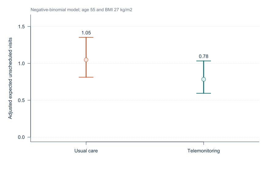
An IRR gives a relative effect. Predicted counts or rates for representative profiles provide absolute context. A 50% rate reduction has different clinical implications when the baseline rate is 0.1 versus 10 events per person-year.

Negative-binomial parameterisations

Software can express dispersion using $\alpha$ or a size parameter $\theta=1/\alpha$. State the parameterisation so the reported value can be interpreted and reproduced.

Worked example

Reproducible R analysis

make_hypertension_data <- function(n = 180) {
  set.seed(4583)
  i <- seq_len(n)

  data <- data.frame(
    participant_id = sprintf("H%03d", i),
    age = round(runif(n, 30, 80)),
    male = rbinom(n, 1, 0.5),
    bmi = pmin(pmax(round(rnorm(n, 27, 3.5), 1), 18), 40),
    physical_activity = round(runif(n, 2, 7), 1),
    telemonitoring = rbinom(n, 1, 0.5)
  )

  data$adherence <- 4 + runif(n, 0, 5) -
    0.015 * (data$age - 55) + 0.4 * data$telemonitoring
  data$baseline_sbp <- 92 + 0.52 * data$age + 0.85 * data$bmi +
    2.8 * data$male - 1.3 * data$physical_activity + rnorm(n, 0, 4)
  data$followup_sbp <- 58 + 0.47 * data$baseline_sbp +
    0.10 * data$age + 0.52 * data$bmi - 2.0 * data$adherence +
    2.0 * data$male - 4.5 * data$telemonitoring -
    0.55 * data$telemonitoring * (data$bmi - 27) +
    0.006 * (data$age - 55)^2 + rnorm(n, 0, 5)

  data
}

hypertension <- make_hypertension_data()

mean_count <- exp(
  0.25 +
    0.018 * (hypertension$age - 55) +
    0.055 * (hypertension$bmi - 27) -
    0.45 * hypertension$telemonitoring
)

hypertension$visits <- rnbinom(
  nrow(hypertension),
  mu = mean_count,
  size = 3.2
)

poisson_fit <- glm(
  visits ~ telemonitoring + age + bmi,
  data = hypertension,
  family = poisson(link = "log")
)

dispersion <- sum(
  residuals(poisson_fit, type = "pearson")^2
) / df.residual(poisson_fit)

negative_binomial_fit <- MASS::glm.nb(
  visits ~ telemonitoring + age + bmi,
  data = hypertension
)

exp(coef(poisson_fit))
exp(confint.default(poisson_fit))
dispersion

exp(coef(negative_binomial_fit))
exp(confint.default(negative_binomial_fit))
negative_binomial_fit$theta

Cleaned R output

Model              Telemonitoring IRR   95% CI          Dispersion
Poisson                   0.727          0.545 to 0.972   Pearson ratio 1.51
Negative binomial         0.747          0.519 to 1.076   alpha about 0.47

Base R provides Poisson regression through glm(), while MASS provides glm.nb() [2], [3].

Interpreting the output

Presenting the results

Present event counts, exposure time where relevant, rate ratios, confidence intervals and the selected dispersion model.

Visualising adjusted expected counts

Suggested reporting

Zero inflation and recurrent events MMed extension

Many zeros do not automatically require a zero-inflated model. Compare the observed zero frequency with that predicted by a suitable count model and consider whether a separate structural-zero process is scientifically plausible.

Repeated events within participants may require frailty, mixed, GEE or recurrent-event methods.

Common mistakes

Knowledge check

What does an IRR of 0.747 mean?

Answer and reasoning

The expected event rate is estimated to be 0.747 times as high, or about 25% lower, conditional on the model. The confidence interval includes no association.

Why include an offset?

Answer and reasoning

It accounts for differing exposure time while fixing its coefficient at one.

What is overdispersion?

Answer and reasoning

Outcome variability exceeds the Poisson mean–variance assumption, often making Poisson uncertainty too small.

Does a high zero count require a zero-inflated model?

Answer and reasoning

No. The excess must be evaluated relative to the fitted count distribution and a plausible data-generating process.

Why can negative binomial confidence intervals be wider?

Answer and reasoning

The model estimates extra heterogeneity beyond the Poisson variance.

Key take-home messages

References

1. Lawless JF. Negative binomial and mixed Poisson regression. Can J Stat. 1987;15(3):209–225. https://doi.org/10.2307/3314912
2. R Core Team. Fitting generalized linear models. R documentation, package stats version 4.6.1. Vienna: R Foundation for Statistical Computing; 2026. https://stat.ethz.ch/R-manual/R-devel/library/stats/html/glm.html
3. Ripley B, Venables B. MASS: support functions and datasets for Venables and Ripley’s MASS. R package version 7.3-66. 2026. https://doi.org/10.32614/CRAN.package.MASS
4. Hilbe JM. Negative binomial regression. 2nd ed. Cambridge: Cambridge University Press; 2011. https://doi.org/10.1017/CBO9780511973420