Propensity Score Methods

Overview

The propensity score is the probability of receiving treatment conditional on measured baseline covariates [1].

It can be used to construct treated and untreated groups with similar measured covariate distributions.

Common methods are:

• matching;
• inverse-probability weighting;
• stratification;
• covariate adjustment;
• overlap weighting.

Propensity methods do not remove unmeasured confounding.

Why this matters

Ordinary regression can adjust for measured covariates, but treatment and control populations may have poor overlap.

Propensity diagnostics make the design problem visible before outcome modelling.

A well-balanced weighted sample can support a clearer treatment contrast, but only under causal assumptions.

When to use this method

Use propensity methods for observational treatment comparisons when:

• treatment is binary or extendable to multiple levels;
• baseline confounders are measured before treatment;
• sufficient overlap exists;
• the target population and estimand are explicit.

Do not use post-treatment variables in the propensity model.

Research question and variables

The average treatment effect, ATE, asks:

What would the mean outcome difference be if the target population received treatment versus no treatment?

The propensity score is:

ATE weights are:

$$w_i= \frac{A_i}{e(X_i)} + \frac{1-A_i}{1-e(X_i)}$$

Stabilised weights replace numerator 1 with the marginal treatment probability.

Data structure

Propensity-score variables

simulated data

Variable	Role
treatment	Exposure or treatment
age	Baseline confounder
severity	Baseline confounder
comorbidity	Baseline confounder
outcome	Post-treatment outcome

Statistical assumptions

Propensity-score strategies

Matching

Pairs or sets participants with similar scores.

The estimand depends on the matched population.

Weighting

Creates a pseudo-population representing ATE, ATT or overlap targets.

Stratification

Compares treatment within score strata and combines estimates.

Regression adjustment

Includes the score in an outcome model, but one-dimensional adjustment may not achieve balance.

Worked example

Worked analysis in R

causal_data <- read.csv(
  "data/part-16-causal-data.csv"
)

propensity_fit <- glm(
  treatment ~ age +
    severity +
    comorbidity,
  data = causal_data,
  family = binomial
)

causal_data$ps <- predict(
  propensity_fit,
  type = "response"
)

treated_prevalence <- mean(
  causal_data$treatment
)

causal_data$stabilised_weight <- ifelse(
  causal_data$treatment == 1,
  treated_prevalence /
    causal_data$ps,
  (1 - treated_prevalence) /
    (1 - causal_data$ps)
)

weighted_fit <- lm(
  outcome ~ treatment,
  data = causal_data,
  weights = stabilised_weight
)

summary(weighted_fit)
confint(weighted_fit)

# Recommended implementation
# WeightIt::weightit(...)
# cobalt::bal.tab(...)
# cobalt::love.plot(...)

Selected analysis output

Stabilised IPTW treatment effect is approximately -3.51 outcome units (95% CI -3.89 to -3.13).

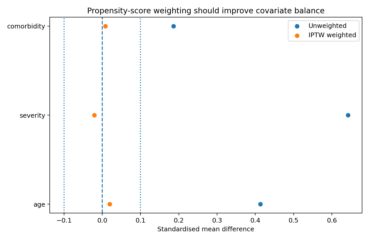
Post-weighting standardised differences are closer to zero than unweighted differences.

Visualising covariate balance

Overlap and extreme weights

Poor overlap occurs when some patients almost always or almost never receive treatment.

Extreme weights increase variance and sensitivity to model misspecification.

Options include:

• trimming;
• truncation;
• overlap weights;
• changing the target population;
• reporting non-identifiability.

These choices change the estimand and must be prespecified or disclosed.

Outcome analysis

Weighted outcome models should use robust or design-aware variance.

Matching requires paired or cluster-aware analysis.

Doubly robust estimators combine propensity and outcome models, but they are not robust to unmeasured confounding.

Interpreting the output

Presenting the results

Suggested reporting

Report covariate selection, model form, score distributions, overlap, balance before and after design, weight diagnostics, estimand, outcome model and sensitivity analyses [2], [3].

The cobalt package provides complementary balance tables and plots for propensity-score designs [4].

Common mistakes

Knowledge check

What is the propensity score?

Answer and reasoning

The conditional probability of treatment given measured baseline covariates.

What is the main diagnostic target?

Answer and reasoning

Measured-covariate balance and overlap.

Does weighting remove unmeasured confounding?

Answer and reasoning

No.

Why are extreme weights problematic?

Answer and reasoning

They create unstable estimates and signal limited positivity.

What changes when trimming patients?

Answer and reasoning

The target population and estimand.

Key take-home messages

References

1. Rosenbaum PR, Rubin DB. The central role of the propensity score. Biometrika. 1983;70(1):41–55. https://doi.org/10.1093/biomet/70.1.41
2. Austin PC. An introduction to propensity score methods. Multivariate Behav Res. 2011;46(3):399–424. https://doi.org/10.1080/00273171.2011.568786
3. Greifer N. WeightIt: weighting for covariate balance in observational studies. R package. https://CRAN.R-project.org/package=WeightIt
4. Greifer N. cobalt: covariate balance tables and plots. R package. https://CRAN.R-project.org/package=cobalt