
Part 7 · Module 2
Comparing Two Independent Proportions
Learn how to compare binary outcomes in two independent groups using risk difference, risk ratio, odds ratio, confidence intervals and reproducible R code.
Learning outcomes
After completing this lecture, you should be able to:
- Recognise two independent binary-outcome groups.
- Calculate and interpret risk difference, risk ratio and odds ratio.
- Distinguish absolute and relative measures of association.
- Calculate confidence intervals and a two-sided test for independent proportions.
- Explain why an odds ratio is not a risk ratio.
- Use reproducible R code to produce a complete two-group categorical analysis.
Overview
A binary outcome has two states, such as:
- controlled or uncontrolled;
- event or no event;
- response or no response;
- infected or not infected.
When the two groups contain different independent participants, the group proportions can be compared using absolute and relative effect measures.
The most common measures are:
- risk difference, also called proportion difference;
- risk ratio, also called relative risk in appropriate designs;
- odds ratio.
These measures answer different questions and should be selected according to the design and estimand [3]. A complete analysis should select the primary effect measure according to the study design and clinical objective rather than reporting whichever value appears most impressive.
Why this matters
Suppose blood-pressure control is achieved by:
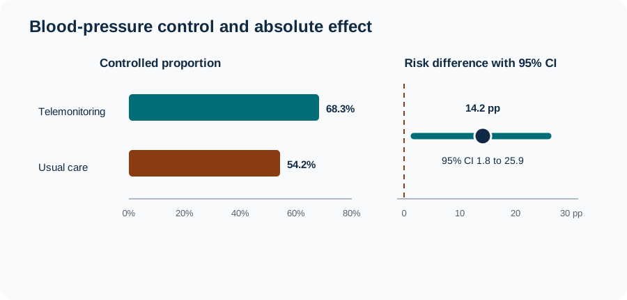
- 68.3% of participants receiving telemonitoring;
- 54.2% receiving usual care.
The same data can be described as:
- risk difference 14.2 percentage points;
- risk ratio 1.26;
- odds ratio 1.83.
These values are not interchangeable.
The risk difference communicates the additional proportion controlled. The risk ratio communicates relative probability. The odds ratio compares odds and can appear farther from one when the outcome is common.
Confidence intervals for differences between independent proportions require appropriate methods. Newcombe compared several interval procedures and demonstrated limitations of simple Wald approaches [1].
When to use this method
Use an independent two-proportion comparison when:
- the outcome is binary;
- each participant belongs to exactly one group;
- one known outcome is contributed per participant;
- participants are independent across groups;
- and the group-specific denominators are defined.
Do not use it for:
- paired before-and-after outcomes;
- matched participants;
- repeated visits;
- clustered randomisation without cluster-aware inference;
- person-time rates;
- or case–control data when risks cannot be estimated from the sampling design.
Research question and variables
Let:
- be the probability of control with telemonitoring;
- be the probability of control with usual care.
The risk difference is:
The risk ratio is:
The odds ratio is:
The null values are:
- 0 for the risk difference;
- 1 for the risk ratio;
- 1 for the odds ratio.
Data structure
Two-by-two table for independent groups
simulated dataTable 1. Blood-pressure control by treatment group
| Group | Controlled | Not controlled | Total |
|---|---|---|---|
| Telemonitoring | 82 | 38 | 120 |
| Usual care | 65 | 55 | 120 |
Note: Rows are independent treatment groups. All counts are simulated.
The row and column orientation should be fixed before calculating effect measures.
Statistical assumptions
In a randomised trial, intention-to-treat analysis commonly retains participants according to allocated group. Missing binary outcomes still require a prespecified strategy.
In an observational comparison, a crude two-by-two analysis does not control confounding or justify a causal interpretation [4].
How the method works
Group risks
Risk difference
Risk ratio
Odds ratio
Worked example
Reproducible R analysis
x_t <- 82
n_t <- 120
x_u <- 65
n_u <- 120

p_t <- x_t / n_t
p_u <- x_u / n_u

risk_difference <- p_t - p_u
risk_ratio <- p_t / p_u
odds_ratio <- (x_t * (n_u - x_u)) /
  ((n_t - x_t) * x_u)

wilson_ci <- function(x, n, conf.level = 0.95) {
  z <- qnorm(1 - (1 - conf.level) / 2)
  p <- x / n
  den <- 1 + z^2 / n
  centre <- (p + z^2 / (2 * n)) / den
  half <- z / den * sqrt(
    p * (1 - p) / n + z^2 / (4 * n^2)
  )
  c(lower = centre - half, upper = centre + half)
}

# Newcombe interval for independent risk difference
ci_t <- wilson_ci(x_t, n_t)
ci_u <- wilson_ci(x_u, n_u)

rd_ci <- c(
  lower = unname(risk_difference - sqrt(
    (p_t - ci_t["lower"])^2 +
      (ci_u["upper"] - p_u)^2
  )),
  upper = unname(risk_difference + sqrt(
    (ci_t["upper"] - p_t)^2 +
      (p_u - ci_u["lower"])^2
  ))
)

rr_se <- sqrt(
  1 / x_t - 1 / n_t +
    1 / x_u - 1 / n_u
)
rr_ci <- exp(log(risk_ratio) + c(-1, 1) * 1.96 * rr_se)

or_se <- sqrt(
  1 / x_t + 1 / (n_t - x_t) +
    1 / x_u + 1 / (n_u - x_u)
)
or_ci <- exp(log(odds_ratio) + c(-1, 1) * 1.96 * or_se)

test <- prop.test(
  x = c(x_t, x_u),
  n = c(n_t, n_u),
  correct = FALSE
)

z_statistic <- sign(risk_difference) * sqrt(unname(test$statistic))

output <- data.frame(
  telemonitoring_percent = 100 * p_t,
  usual_care_percent = 100 * p_u,
  risk_difference_pp = 100 * risk_difference,
  rd_lower_pp = 100 * unname(rd_ci["lower"]),
  rd_upper_pp = 100 * unname(rd_ci["upper"]),
  risk_ratio = risk_ratio,
  rr_lower = unname(rr_ci[1]),
  rr_upper = unname(rr_ci[2]),
  odds_ratio = odds_ratio,
  or_lower = unname(or_ci[1]),
  or_upper = unname(or_ci[2]),
  z = z_statistic,
  p_value = test$p.value
)

round(output, 3)
Cleaned R output
 telemonitoring_percent usual_care_percent risk_difference_pp rd_lower_pp rd_upper_pp risk_ratio rr_lower rr_upper odds_ratio or_lower or_upper     z p_value
                 68.333             54.167             14.167       1.843      25.903      1.262    1.028    1.548      1.826    1.079    3.090 2.252   0.024
Base R’s prop.test() implements a score-type comparison of proportions and can apply a continuity correction [2]. The lecture uses correct = FALSE and reports this choice explicitly.
Interpreting the output
Presenting the results
Table 2. Blood-pressure control by group
| Group | Controlled / total | Proportion |
|---|---|---|
| Telemonitoring | 82 / 120 | 68.3% |
| Usual care | 65 / 120 | 54.2% |
Risk difference 14.2 percentage points (95% CI 1.8 to 25.9); risk ratio 1.26 (95% CI 1.03 to 1.55); .
Suggested reporting
Why confidence-interval methods differ MMed extension
A Wald interval for the risk difference uses a symmetric normal approximation. Its coverage can be poor with small samples or extreme proportions.
Newcombe’s method combines Wilson intervals from the two groups and often provides improved coverage [1].
Regression or standardisation is preferable when adjusted risk differences or risk ratios are required.
Common mistakes
Knowledge check
Why are the two groups independent?
Answer and reasoning
Each participant belongs to one allocated group and contributes one outcome. No participant is paired or repeated across the two rows.
What does the risk difference of 14.2 percentage points mean?
Answer and reasoning
The estimated probability of control is 0.142 higher with telemonitoring, equivalent to approximately 14 additional controlled participants per 100 under comparable conditions.
Does an odds ratio of 1.83 mean the probability is 83% higher?
Answer and reasoning
No. It means the odds are 1.83 times as high. When the outcome is common, the odds ratio can differ materially from the risk ratio.
Can a case–control study estimate the risk ratio directly from sampled case and control counts?
Answer and reasoning
Usually not, because the investigators determine the numbers of cases and controls. The sampled proportions do not represent population risks, although the odds ratio can be estimated under suitable assumptions.
Why should absolute and relative effects both be considered?
Answer and reasoning
A relative effect can correspond to very different absolute benefits depending on baseline risk. Absolute effects are essential for clinical and service decisions.
Key take-home messages
References
- Newcombe RG. Interval estimation for the difference between independent proportions: comparison of eleven methods. Stat Med. 1998;17(8):873–890. https://doi.org/10.1002/(SICI)1097-0258(19980430)17:8%3C873::AID-SIM779%3E3.0.CO;2-I
- R Core Team. Test of equal or given proportions. R documentation, package stats version 4.6.1. Vienna: R Foundation for Statistical Computing; 2026. https://stat.ethz.ch/R-manual/R-devel/library/stats/html/prop.test.html
- Agresti A. Categorical data analysis. 3rd ed. Hoboken (NJ): Wiley; 2013.
- Lash TL, VanderWeele TJ, Haneuse S, Rothman KJ. Modern epidemiology. 4th ed. Philadelphia: Wolters Kluwer; 2021.
These notes support learning and research planning and do not replace statistical consultation for a specific study.