Bland-Altman Analysis

Overview

Bland–Altman analysis evaluates agreement between two numerical measurement methods using their paired differences [1].

It estimates:

• average bias;
• variability of individual differences;
• 95% limits of agreement;
• patterns of disagreement across the measurement range.

The method does not declare methods interchangeable automatically.

Clinical or technical acceptability limits must be specified independently.

Why this matters

Correlation and regression can show a strong relationship while methods differ systematically.

A paired t-test can detect average bias but says little about the spread of individual differences.

Bland–Altman analysis asks:

For most participants, how far apart are the two methods likely to be?

That question is directly relevant when replacing a device, laboratory assay, observer or measurement protocol.

When to use Bland–Altman analysis

Use the method when:

• two methods measure the same continuous quantity;
• the same participants receive both methods;
• one paired difference per independent participant is available;
• absolute interchangeability is the question.

Extensions are required for:

• repeated measurements per participant;
• several observers;
• replicate readings;
• non-constant variance;
• non-normal differences;
• reference methods with negligible error.

Research question and variables

For participant $i$:

$$d_i=B_i-A_i$$

and:

$$m_i=\frac{A_i+B_i}{2}$$

The sign convention must be stated.

Reversing the subtraction reverses bias and limits.

Data structure

Bland–Altman variables

simulated data

Variable	Meaning
method_a	First measurement
method_b	Second measurement
difference	Method B minus Method A
pair_mean	Mean of both methods
id	Independent participant

The plot uses pair mean on the horizontal axis and difference on the vertical axis.

Statistical assumptions

How the method works

Mean bias is:

If differences are approximately normal with constant variance:

Approximately 95% of future paired differences from a comparable population are expected within these limits under the model.

The limits are estimates and have their own confidence intervals.

Worked example

Worked analysis in R

Download the lecture dataset using the Dataset link on this page and save it in the R working directory before running the code.

measurement_data <- read.csv(
  "part-12-continuous-measurement-data.csv"
)

measurement_data$difference <- with(
  measurement_data,
  method_b - method_a
)

measurement_data$pair_mean <- with(
  measurement_data,
  (method_a + method_b) / 2
)

n <- nrow(measurement_data)
bias <- mean(
  measurement_data$difference
)

sd_difference <- sd(
  measurement_data$difference
)

limits <- bias + c(-1, 1) *
  1.96 * sd_difference

bias_ci <- bias + c(-1, 1) *
  qt(0.975, df = n - 1) *
  sd_difference / sqrt(n)

se_limit <- sd_difference *
  sqrt(
    1 / n +
    1.96^2 / (2 * (n - 1))
  )

limit_ci <- rbind(
  lower = limits[1] + c(-1, 1) *
    qt(0.975, df = n - 1) *
    se_limit,
  upper = limits[2] + c(-1, 1) *
    qt(0.975, df = n - 1) *
    se_limit
)

proportional_bias <- lm(
  difference ~ pair_mean,
  data = measurement_data
)

c(
  bias = bias,
  lower_limit = limits[1],
  upper_limit = limits[2]
)

bias_ci
limit_ci
summary(proportional_bias)

plot(
  measurement_data$pair_mean,
  measurement_data$difference,
  xlab = "Mean of Method A and Method B",
  ylab = "Method B minus Method A"
)

abline(
  h = c(
    bias,
    limits
  ),
  lty = c(1, 2, 2)
)

Selected analysis output

Mean difference = 10.214
95% CI for bias = 9.990 to 10.438

Lower limit = 7.401
Approximate 95% CI = 7.018 to 7.785

Upper limit = 13.026
Approximate 95% CI = 12.643 to 13.410

Difference-versus-mean slope = 0.042
p < 0.001

Visualising agreement

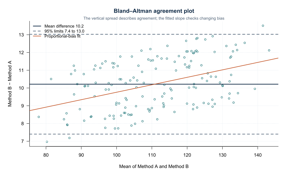
The plot suggests a small positive proportional trend in differences.

The clinical importance of this trend depends on the scale and range.

Proportional bias

Regression of differences on pair means can describe systematic change in bias across the range.

A small p-value does not automatically establish clinically important proportional bias.

Inspect:

• slope magnitude;
• confidence interval;
• graph;
• measurement range;
• pre-established tolerance.

Because the pair mean contains both measurements, ordinary regression has limitations. More advanced errors-in-variables approaches may be considered [2].

Heteroscedasticity

If variability increases with measurement magnitude, ordinary additive limits can be misleading.

Options include:

• logarithmic transformation;
• ratio or percentage differences;
• regression-based limits;
• variance modelling.

For log-transformed data, back-transformed limits are multiplicative ratios.

Example interpretation:

Method B values are expected to lie between 0.90 and 1.18 times Method A values for approximately 95% of comparable measurements.

Normality and outliers

Limits based on $1.96s_d$ assume approximately normal differences.

Normality of the original methods is not required.

Inspect the difference distribution and outliers.

Robust or non-parametric limits may be considered, but they require sufficient sample size and transparent interpretation.

Repeated measurements

When each participant contributes repeated pairs, differences are correlated.

Ordinary limits treating every pair as independent are too precise.

Use methods that separate:

• between-participant variation;
• within-participant measurement error;
• replicate-level variation.

Bland and Altman describe extensions for repeated method-comparison data [3].

Interpreting the output

Presenting the results

Suggested reporting

Report subtraction direction, bias, SD of differences, limits with uncertainty, clinically acceptable limits, plot, heteroscedasticity, proportional bias, outliers and repeated-measurement structure.

A modern practical guideline also recommends reporting both Bland–Altman agreement and an appropriately specified ICC when they answer complementary questions [4]. An accessible clinical explanation of the plot and its limitations is provided by Giavarina [5].

Common mistakes

Knowledge check

What does the mean difference measure?

Answer and reasoning

Average systematic bias between the two methods using the stated subtraction direction.

What do the 95% limits of agreement describe?

Answer and reasoning

The range expected to contain approximately 95% of individual paired differences in a comparable population under the assumptions.

Do limits of agreement determine clinical acceptability?

Answer and reasoning

No. Acceptable limits must be specified using clinical or technical requirements.

What suggests a log transformation may be useful?

Answer and reasoning

Difference variability increasing with measurement magnitude or multiplicative error.

Why are ordinary limits invalid for repeated pairs from one participant?

Answer and reasoning

The differences are correlated and do not provide independent information.

Key take-home messages

References

1. Bland JM, Altman DG. Statistical methods for assessing agreement between two methods of clinical measurement. Lancet. 1986;1(8476):307–310. https://doi.org/10.1016/S0140-6736(86)90837-8
2. Francq BG, Govaerts BB. How to regress and predict in a Bland–Altman plot? Review and contribution based on tolerance intervals and correlated-errors-in-variables models. Stat Med. 2016;35(14):2328–2358. https://doi.org/10.1002/sim.6872
3. Bland JM, Altman DG. Measuring agreement in method comparison studies. Stat Methods Med Res. 1999;8(2):135–160. https://doi.org/10.1177/096228029900800204
4. Haghayegh S, Kang HA, Khoshnevis S, Smolensky MH, Diller KR. A comprehensive guideline for Bland–Altman and intraclass correlation calculations. Physiol Meas. 2020;41(5):055012. https://doi.org/10.1088/1361-6579/ab86d6
5. Giavarina D. Understanding Bland Altman analysis. Biochem Med (Zagreb). 2015;25(2):141–151. https://doi.org/10.11613/BM.2015.015