Comparing Diagnostic Tests

Overview

Comparing diagnostic tests requires direct comparison of their performance.

It is not sufficient to report:

• Test A sensitivity is significant;
• Test B sensitivity is not significant;
• therefore, Test A is better.

The difference between tests must be estimated and tested directly.

The analysis depends on whether the tests are:

• paired: both tests applied to the same participants;
• unpaired: different participant samples.

Paired designs are efficient because participant difficulty and disease status are shared, but the correlation must be represented.

Why this matters

Two tests can differ in:

• sensitivity;
• specificity;
• predictive values;
• likelihood ratios;
• AUC;
• failed or indeterminate results;
• cost, burden and safety;
• downstream consequences.

A test with higher AUC may have worse sensitivity at the threshold needed for triage.

A comparison should therefore begin with the intended clinical role and primary metric.

When to compare tests

Use a formal comparison when the objective is to determine whether a new test:

• is superior;
• is non-inferior;
• improves an existing pathway;
• replaces another test;
• adds value after another test;
• has acceptable trade-offs.

Define the primary metric before data analysis.

Research question and variables

The paired design contains:

• one disease status per participant;
• two test results per participant;
• matched classification errors.

For sensitivity, analysis is restricted to diseased participants.

For specificity, analysis is restricted to non-diseased participants.

For AUC, both continuous scores and the shared disease status are used.

Data structure

Paired test data

simulated data

Variable	Meaning
id	Pairing identifier
disease	Shared target-condition status
score_a, score_b	Continuous paired test values
test_a_positive, test_b_positive	Paired binary classifications

Dropping the participant identifier would prevent valid paired analysis.

Statistical assumptions

Comparing paired sensitivity

Among diseased participants, compare whether each test is positive.

Only discordant pairs inform the difference:

• Test A positive, Test B negative;
• Test A negative, Test B positive.

In the simulated study:

• 24 diseased participants are positive only on Test A;
• none are positive only on Test B.

The paired sensitivity difference is:

$$84.2\%-64.2\%=20.0\text{ percentage points}$$

An exact McNemar-type binomial test uses the discordant-pair principle introduced for correlated proportions [1] and gives:

$$p<0.001$$

Comparing paired specificity

Among non-diseased participants, compare whether each test is negative.

The discordant correct-negative counts are:

• Test A specific only: 2;
• Test B specific only: 36.

The specificity difference is:

$$75.0\%-87.1\%=-12.1\text{ percentage points}$$

The paired exact test gives:

$$p<0.001$$

Test A is more sensitive but less specific at the selected thresholds.

Comparing AUC

For paired continuous tests, AUC estimates are correlated.

DeLong’s method estimates the variance of the paired AUC difference non-parametrically [2].

The simulated results are:

• Test A AUC 0.895;
• Test B AUC 0.857;
• difference 0.037;
• 95% CI 0.019 to 0.055;
• $p<0.001$.

The AUC comparison favours Test A overall, but it does not resolve the threshold-specific clinical trade-off.

Worked example

Worked analysis in R

make_diagnostic_data <- function(n = 400) {
  id <- seq_len(n)
  age <- 20 + ((7 * id) %% 61)
  male <- as.integer(id %% 2 == 0)

  disease <- as.integer(
    ((id * 37) %% 100) < 30
  )

  score_a <-
    47 +
    11 * disease +
    0.08 * (age - 50) +
    7.5 * sin(id * 1.13) +
    3.5 * cos(id * 0.37)

  score_b <-
    48 +
    9 * disease +
    0.05 * (age - 50) +
    7.2 * sin(id * 1.13 + 0.45) +
    4.0 * cos(id * 0.37 + 0.20)

  disease_rank <- (id * 43) %% 100
  nondisease_rank <- (id * 47) %% 100

  reference_positive <- ifelse(
    disease == 1,
    disease_rank < 88,
    nondisease_rank >= 95
  )

  data.frame(
    id = id,
    age = age,
    male = male,
    disease = disease,
    score_a = score_a,
    score_b = score_b,
    reference_positive = as.integer(
      reference_positive
    )
  )
}

diagnostic_data <- make_diagnostic_data()

cutoff_a <- 51.962318662698785
cutoff_b <- 55.26626112612387

diagnostic_data$test_a_positive <- as.integer(
  diagnostic_data$score_a >= cutoff_a
)

diagnostic_data$test_b_positive <- as.integer(
  diagnostic_data$score_b >= cutoff_b
)

library(pROC)

# Paired sensitivity comparison among diseased participants
diseased <- diagnostic_data[
  diagnostic_data$disease == 1,
]

sensitivity_discordant <- table(
  Test_A = diseased$test_a_positive,
  Test_B = diseased$test_b_positive
)

sensitivity_test <- mcnemar.test(
  sensitivity_discordant,
  correct = FALSE
)

sensitivity_exact <- binom.test(
  x = sensitivity_discordant["1", "0"],
  n = sensitivity_discordant["1", "0"] +
    sensitivity_discordant["0", "1"],
  p = 0.5
)

# Paired specificity comparison among non-diseased participants
non_diseased <- diagnostic_data[
  diagnostic_data$disease == 0,
]

specificity_discordant <- table(
  Test_A_negative =
    1 - non_diseased$test_a_positive,
  Test_B_negative =
    1 - non_diseased$test_b_positive
)

specificity_exact <- binom.test(
  x = specificity_discordant["1", "0"],
  n = specificity_discordant["1", "0"] +
    specificity_discordant["0", "1"],
  p = 0.5
)

roc_a <- roc(
  diagnostic_data$disease,
  diagnostic_data$score_a,
  levels = c(0, 1),
  direction = "<"
)

roc_b <- roc(
  diagnostic_data$disease,
  diagnostic_data$score_b,
  levels = c(0, 1),
  direction = "<"
)

auc_comparison <- roc.test(
  roc_a,
  roc_b,
  paired = TRUE,
  method = "delong"
)

sensitivity_discordant
specificity_discordant
sensitivity_exact
specificity_exact
auc_comparison

Selected analysis output

Sensitivity discordance among diseased participants
Test A positive only = 24
Test B positive only = 0
Exact paired p < 0.001

Specificity discordance among non-diseased participants
Test A specific only = 2
Test B specific only = 36
Exact paired p < 0.001

Paired AUC difference = 0.037
95% CI = 0.019 to 0.055
DeLong p < 0.001

Packages such as DTComPair and testCompareR provide additional paired comparisons for binary diagnostic tests [4], [5].

Visualising paired performance

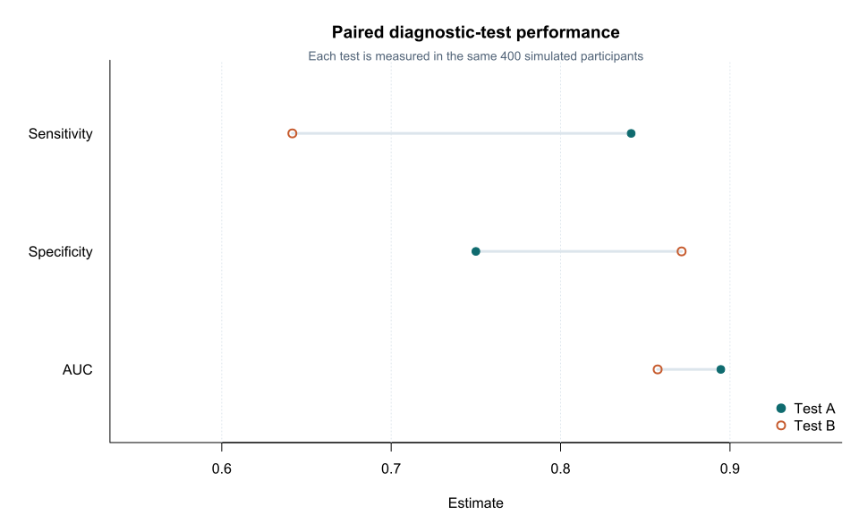
The figure should not replace paired difference estimates and confidence intervals.

Predictive-value comparison

PPV and NPV comparisons in paired designs are more complex because test-positive and test-negative denominators differ between tests.

Ordinary independent-proportion tests are inappropriate.

Use methods designed for paired predictive values, and interpret results at the observed prevalence and testing pathway.

Likelihood-ratio comparison

Likelihood ratios share sensitivity and specificity estimates.

Comparing them requires methods that reflect the joint paired structure.

A test can have a higher $LR+$ but a worse $LR-$.

Report both and focus on clinically relevant probability updating.

Non-inferiority

A new test may offer:

• lower cost;
• faster turnaround;
• lower burden;
• greater accessibility.

The objective may be to show that sensitivity is no worse than the comparator by more than a prespecified margin.

The margin must be justified clinically and defined before analysis.

Failure to find superiority does not establish non-inferiority.

Multiplicity

Testing:

• sensitivity;
• specificity;
• PPV;
• NPV;
• AUC;
• many thresholds;
• many subgroups

creates multiple opportunities for favourable findings.

Identify the primary metric and treat other comparisons as secondary or exploratory.

Interpreting the output

Presenting the results

Suggested reporting

Report paired or unpaired design, thresholds, primary metric, difference estimates with confidence intervals, discordant counts, AUC method, multiplicity strategy and clinical consequences.

Common mistakes

Knowledge check

Which observations inform the paired sensitivity comparison?

Answer and reasoning

Diseased participants whose two test classifications disagree.

Why is the DeLong comparison paired?

Answer and reasoning

Both scores are measured in the same participants and share disease status.

Does larger AUC guarantee higher sensitivity at the chosen threshold?

Answer and reasoning

No. AUC summarises all thresholds, while sensitivity depends on one operating point.

Can non-significant superiority establish non-inferiority?

Answer and reasoning

No. Non-inferiority requires a prespecified margin and dedicated analysis.

Why can one test be preferred despite lower specificity?

Answer and reasoning

Its clinical role may prioritise avoiding missed disease, with false positives resolved by confirmatory testing.

Key take-home messages

References

1. McNemar Q. Note on the sampling error of the difference between correlated proportions or percentages. Psychometrika. 1947;12(2):153–157. https://doi.org/10.1007/BF02295996
2. DeLong ER, DeLong DM, Clarke-Pearson DL. Comparing the areas under two or more correlated receiver operating characteristic curves: a nonparametric approach. Biometrics. 1988;44(3):837–845. https://doi.org/10.2307/2531595
3. Pepe MS. The statistical evaluation of medical tests for classification and prediction. Oxford: Oxford University Press; 2003. https://doi.org/10.1093/oso/9780198565826.001.0001
4. Stock C, Hielscher T. DTComPair: comparison of binary diagnostic tests in a paired study design. R package version 1.2.6. 2024. https://CRAN.R-project.org/package=DTComPair
5. Wilson KJ, Henrion M, Roldán-Nofuentes JA. testCompareR: comparing two diagnostic tests with dichotomous results using paired data. R package version 1.1.1. 2024. https://doi.org/10.32614/CRAN.package.testCompareR