
Part 7 · Module 5
Ordinal Categorical Data
Learn how to preserve and analyse ordered outcome categories using cumulative distributions, proportional-odds models and reproducible R output.
Learning outcomes
After completing this lecture, you should be able to:
- Distinguish ordinal from nominal categorical outcomes.
- Present ordinal outcomes using category and cumulative proportions.
- Explain why arbitrary numerical category codes are not measured quantities.
- Interpret a proportional-odds odds ratio on the correct cumulative scale.
- Assess the plausibility of the proportional-odds assumption.
- Use reproducible R code to fit and report a simple ordinal logistic model.
Overview
An ordinal categorical variable has categories with a meaningful order but without known equal distances between adjacent categories.
Examples include:
- no, mild, moderate or marked improvement;
- disease stage I, II, III or IV;
- never, sometimes, often or always;
- no limitation, some limitation or severe limitation;
- ordered toxicity grades.
Ordinal data contain more information than nominal categories because order is known. They contain less quantitative information than measured numerical outcomes because the distance between categories is not established.
The analysis should preserve the ordering where practical. Dichotomising an ordinal outcome can discard information and make results depend on an arbitrary cut-off.
Why this matters
Coding categories as:
- none = 0;
- mild = 1;
- moderate = 2;
- marked = 3
does not prove that the distance from none to mild equals the distance from moderate to marked.
A mean of these codes may be convenient but requires a substantive interpretation that is often absent.
A general Pearson chi-square test ignores the ordering. It can detect any distributional difference but may be less focused than an ordinal model when the scientific question concerns movement towards higher or lower categories.
The proportional-odds model is a widely used cumulative-link model for ordered outcomes [1], [2].
When to use this method
Use an ordinal analysis when:
- the outcome categories have a scientifically meaningful order;
- every participant contributes one category;
- the full ordered distribution is relevant;
- and the selected model’s assumptions are sufficiently reasonable.
Alternative methods include:
- Pearson chi-square for a general unordered association;
- rank-based methods for probability or distributional contrasts;
- proportional-odds logistic regression;
- partial proportional-odds models;
- adjacent-category or continuation-ratio models;
- repeated ordinal models for longitudinal data.
The model should match how categories arise clinically.
Research question and variables
Let have ordered categories:
corresponding to none, mild, moderate and marked improvement.
The explanatory variable is group:
- usual care;
- intervention.
A proportional-odds model compares the odds of being in a higher rather than lower category across every cumulative threshold using one common group coefficient.
Data structure
Ordered outcome by study group
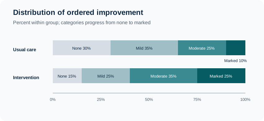
simulated dataTable 1. Improvement category by group
| Group | None | Mild | Moderate | Marked | Total |
|---|---|---|---|---|---|
| Usual care | 30 | 35 | 25 | 10 | 100 |
| Intervention | 15 | 25 | 35 | 25 | 100 |
Note: Categories are ordered from least to greatest improvement. Counts are simulated.
Cumulative percentages at or below each threshold are:
| Group | None or below | Mild or below | Moderate or below |
|---|---|---|---|
| Usual care | 30% | 65% | 90% |
| Intervention | 15% | 40% | 75% |
The intervention distribution is shifted towards higher categories.
Statistical assumptions
Proportional odds
For every threshold , the model assumes the same group coefficient.
In this example, the intervention effect should be broadly similar for:
- mild or higher versus none;
- moderate or higher versus none or mild;
- marked versus lower categories.
Observed threshold-specific odds ratios are approximately:
- 2.43;
- 2.79;
- 3.00.
Their similarity supports, but does not prove, a common proportional-odds summary.
How the method works
One common parameterisation is:
A positive indicates a shift towards higher categories under this parameterisation.
The thresholds vary, but remains common.
Worked example
Reproducible R analysis
The polr() function in the recommended MASS package fits proportional-odds logistic regression [3]. The analysis is designed for R version 4.6.1 [4].
ordinal_counts <- data.frame(
  group = rep(c("Usual care", "Intervention"), each = 4),
  improvement = rep(
    c("None", "Mild", "Moderate", "Marked"),
    times = 2
  ),
  count = c(
    30, 35, 25, 10,
    15, 25, 35, 25
  )
)

ordinal_data <- ordinal_counts[
  rep(seq_len(nrow(ordinal_counts)), ordinal_counts$count),
  c("group", "improvement")
]

ordinal_data$group <- factor(
  ordinal_data$group,
  levels = c("Usual care", "Intervention")
)

ordinal_data$improvement <- ordered(
  ordinal_data$improvement,
  levels = c("None", "Mild", "Moderate", "Marked")
)

fit <- MASS::polr(
  improvement ~ group,
  data = ordinal_data,
  method = "logistic",
  Hess = TRUE
)

beta <- unname(coef(fit)["groupIntervention"])
se <- sqrt(vcov(fit)["groupIntervention", "groupIntervention"])
z <- beta / se
p_value <- 2 * pnorm(-abs(z))

ordinal_or <- exp(beta)
or_ci <- exp(beta + c(-1, 1) * 1.96 * se)

output <- data.frame(
  coefficient = beta,
  standard_error = se,
  z = z,
  p_value = p_value,
  ordinal_odds_ratio = ordinal_or,
  ci_lower = or_ci[1],
  ci_upper = or_ci[2]
)

round(output, 3)
Cleaned R output
 coefficient standard_error     z p_value ordinal_odds_ratio ci_lower ci_upper
       1.000          0.263 3.800 0.000145              2.720    1.623    4.556
Report the p-value as $p<0.001$, not p=0.000.
Displaying the ordered distribution
tab <- with(
  ordinal_data,
  table(group, improvement)
)

round(
  100 * prop.table(tab, margin = 1),
  1
)
improvement
group None Mild Moderate Marked
Usual care 30.0 35.0 25.0 10.0
Intervention 15.0 25.0 35.0 25.0Interpreting the output
Presenting the results
Table 2. Improvement category within each group
| Group | None | Mild | Moderate | Marked |
|---|---|---|---|---|
| Usual care | 30.0% | 35.0% | 25.0% | 10.0% |
| Intervention | 15.0% | 25.0% | 35.0% | 25.0% |
Common cumulative odds ratio 2.72 (95% CI 1.62 to 4.56), .
Suggested reporting
When proportional odds is unsuitable MMed extension
If group effects vary materially across thresholds, alternatives include:
- partial proportional-odds models;
- separate binary cumulative models;
- adjacent-category models;
- continuation-ratio models;
- multinomial logistic regression.
These alternatives estimate more parameters and require sufficient sample information.
Part VIII develops ordinal logistic regression in greater depth.
Common mistakes
Knowledge check
Why is improvement category ordinal rather than numerical?
Answer and reasoning
The categories have a meaningful order, but the distance from none to mild is not known to equal the distance from moderate to marked.
What does the ordinal odds ratio of 2.72 mean?
Answer and reasoning
Under proportional odds, the intervention group’s odds of being in a higher category are estimated to be 2.72 times the usual-care odds across each cumulative threshold.
Does the odds ratio mean marked improvement is 2.72 times as common?
Answer and reasoning
Not directly. The common ordinal odds ratio combines all cumulative thresholds. Category-specific probabilities should be inspected separately.
Why should category percentages accompany the model?
Answer and reasoning
They show the absolute outcome distribution and make the direction and clinical relevance visible. The model estimate alone is not enough.
What should be considered if threshold-specific odds ratios differ greatly?
Answer and reasoning
The proportional-odds assumption may be unsuitable. A partial proportional-odds, multinomial or another ordinal model may be needed.
Key take-home messages
References
- McCullagh P. Regression models for ordinal data. J R Stat Soc Series B Stat Methodol. 1980;42(2):109–127. https://doi.org/10.1111/j.2517-6161.1980.tb01109.x
- Agresti A. Analysis of ordinal categorical data. 2nd ed. Hoboken (NJ): Wiley; 2010. https://doi.org/10.1002/9780470594001
- Venables WN, Ripley BD. Modern applied statistics with S. 4th ed. New York: Springer; 2002. https://doi.org/10.1007/978-0-387-21706-2
- R Core Team. R: a language and environment for statistical computing. Version 4.6.1. Vienna: R Foundation for Statistical Computing; 2026. https://www.R-project.org/
These notes support learning and research planning and do not replace statistical consultation for a specific study.