Simple Linear Regression

Overview

Simple linear regression models the mean of one numerical outcome as a linear function of one predictor:

$$Y_i=\beta_0+\beta_1X_i+\varepsilon_i$$

The slope translates association into clinical units.

Why this matters

Regression provides fitted means, residuals, confidence intervals and prediction intervals. It is directional: reversing outcome and predictor produces a different model. Practical medical-regression interpretation also requires attention to clinical units, design and extrapolation.

When to use this method

Use simple linear regression when the outcome is numerical, one predictor is studied, a linear mean relation answers the question and observations are independent.

Use another method for binary, count, censored, repeated or strongly non-linear outcomes.

Research question and variables

Data structure

Outcome and predictor

simulated data

Variable	Role	Unit
Baseline systolic blood pressure	Outcome	mmHg
Age	Predictor	Years
Participant	Independent unit	One row

Statistical assumptions

How the method works

Ordinary least squares chooses coefficients that minimise squared residuals.

Interpreting the intercept

The intercept is the fitted mean outcome when the predictor equals zero. It is meaningful only when zero is clinically plausible and represented by the data. For adult age, zero years is outside the study population, so the intercept is needed mathematically but should not receive a clinical interpretation.

Centring the predictor changes the reference point without changing the fitted line. If age is centred at 55 years, the intercept becomes the fitted mean blood pressure at age 55. Scaling age in decades changes the slope from a one-year to a ten-year contrast and often improves readability.

Understanding residual variation

The fitted line describes the conditional mean. Individual observations vary around that mean because of biological heterogeneity, measurement error and omitted factors. The residual standard error summarises the typical vertical variation around the line in outcome units.

A small residual standard error relative to clinically relevant differences suggests more precise individual prediction, but it should be interpreted within the observed population. It can change when the sample includes a wider range of disease severity or when measurement quality differs.

Residuals should be plotted against fitted values and the predictor. Curvature suggests that the straight-line form is inadequate. A funnel-shaped pattern suggests non-constant variance. An isolated large residual may represent a data error, a clinically unusual participant or an omitted predictor.

What R-squared does and does not show

$R^2$ is the proportion of sample outcome variation represented by the fitted linear model. It increases when the predictor explains more variation, but it does not show whether the slope is clinically important, unbiased or causal.

A low $R^2$ does not make a slope unimportant. For example, a modest average treatment effect may be clinically useful despite substantial person-to-person variability. Conversely, a high $R^2$ can arise from a strong age pattern without making age an intervention target.

Estimation versus prediction

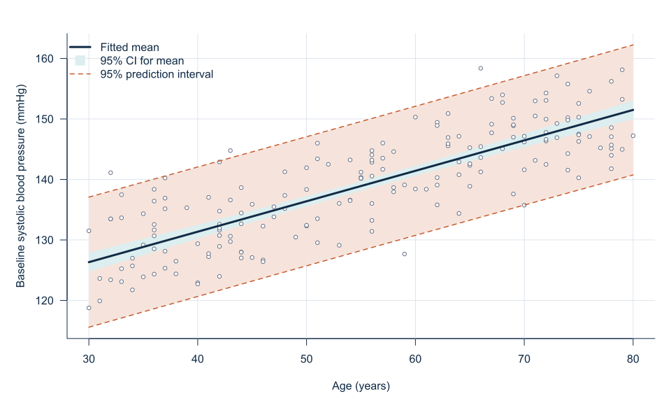
The confidence interval for the slope quantifies uncertainty about the population mean relationship. A confidence interval for the fitted mean at age 60 concerns the average outcome among comparable people aged 60.

An individual prediction interval is wider because a new participant can differ from the fitted mean even if the regression coefficients were known exactly. Clinical prediction requires this individual uncertainty, appropriate validation and predictors available at the intended prediction time.

Extrapolation

A fitted line is supported primarily over the observed predictor range. Extending the equation to children or very old adults would assume that the same linear relation continues beyond the data. Even a visually excellent line within the sample does not justify such extrapolation.

Worked example

Reproducible R analysis

make_hypertension_data <- function(n = 180) {
  set.seed(4583)
  i <- seq_len(n)

  data <- data.frame(
    participant_id = sprintf("H%03d", i),
    age = round(runif(n, 30, 80)),
    male = rbinom(n, 1, 0.5),
    bmi = pmin(pmax(round(rnorm(n, 27, 3.5), 1), 18), 40),
    physical_activity = round(runif(n, 2, 7), 1),
    telemonitoring = rbinom(n, 1, 0.5)
  )

  data$adherence <- 4 + runif(n, 0, 5) -
    0.015 * (data$age - 55) + 0.4 * data$telemonitoring
  data$baseline_sbp <- 92 + 0.52 * data$age + 0.85 * data$bmi +
    2.8 * data$male - 1.3 * data$physical_activity + rnorm(n, 0, 4)
  data$followup_sbp <- 58 + 0.47 * data$baseline_sbp +
    0.10 * data$age + 0.52 * data$bmi - 2.0 * data$adherence +
    2.0 * data$male - 4.5 * data$telemonitoring -
    0.55 * data$telemonitoring * (data$bmi - 27) +
    0.006 * (data$age - 55)^2 + rnorm(n, 0, 5)

  data
}

hypertension <- make_hypertension_data()

fit <- lm(
  baseline_sbp ~ age,
  data = hypertension
)

summary(fit)
confint(fit)

predict(
  fit,
  newdata = data.frame(age = 60),
  interval = "confidence"
)

predict(
  fit,
  newdata = data.frame(age = 60),
  interval = "prediction"
)

Cleaned R output

Term        Estimate   SE      95% CI                p-value
Intercept   111.226    1.554   108.158 to 114.294    <0.001
Age           0.503    0.027     0.450 to 0.557      <0.001

R-squared = 0.659
Residual standard error = 5.391 mmHg

Base R fits linear models using lm() [1].

Interpreting the output

Presenting the results

A confidence interval at age 60 estimates the mean outcome at that age. A prediction interval is wider because it includes individual residual variation.

Present the fitted slope in clinical units, model fit and clinically relevant confidence or prediction intervals.

Visualising the fitted model

Suggested reporting

Centring age MMed extension

Replacing age with age minus 55 leaves the slope and fitted values unchanged but makes the intercept represent expected blood pressure at age 55 [2]. This type of clinically grounded interpretation is central to practical medical regression [3].

Common mistakes

Knowledge check

What does the age slope represent?

Answer and reasoning

It is the expected mean blood-pressure difference associated with a one-year higher age under the linear model.

Why is the intercept not clinically useful?

Answer and reasoning

It refers to age zero, outside the sampled adult range.

Why is a prediction interval wider?

Answer and reasoning

It includes individual residual variation in addition to uncertainty in the mean.

Does R squared prove causation?

Answer and reasoning

No. It describes in-sample linear fit, not a causal proportion.

What should be done if curvature is visible?

Answer and reasoning

Use a defensible non-linear specification rather than forcing one straight slope.

Key take-home messages

References

1. R Core Team. Fitting linear models. R documentation, package stats version 4.6.1. Vienna: R Foundation for Statistical Computing; 2026. https://stat.ethz.ch/R-manual/R-devel/library/stats/html/lm.html
2. Harrell FE Jr. Regression modeling strategies. 2nd ed. Cham: Springer; 2015. https://doi.org/10.1007/978-3-319-19425-7
3. Altman DG. Practical statistics for medical research. London: Chapman and Hall; 1991.