
Part 7 · Module 3
Chi-Square and Fisher's Exact Tests for Contingency Tables
Learn how Pearson's chi-square and Fisher's exact tests analyse contingency tables, with assumption checks, Cramer's V and reproducible R output.
Learning outcomes
After completing this lecture, you should be able to:
- Construct and interpret a contingency table using counts and row or column percentages.
- Explain observed counts, expected counts and Pearson's chi-square statistic.
- Assess the chi-square approximation and choose Fisher's exact test when independent counts are sparse.
- Distinguish a chi-square test of independence from goodness-of-fit and paired analyses.
- Calculate and interpret Cramer's V as an association-strength measure.
- Use reproducible R code to perform and report a contingency-table analysis.
Overview
A contingency table cross-classifies counts according to two categorical variables.
Pearson’s chi-square test can assess whether the row and column variables are statistically independent in the target population under the sampling model [1].
Examples include examining association between:
- treatment group and response category;
- smoking status and disease category;
- clinic type and referral outcome;
- exposure category and adverse-event status.
The test compares observed cell counts with counts expected if the variables were independent.
A chi-square result should not be reported alone; categorical-data interpretation requires the table pattern and meaningful contrasts [3]. The reader also needs:
- the contingency table;
- meaningful percentages;
- the direction and pattern of association;
- an effect-size measure or interpretable contrasts;
- and the denominator.
Why this matters
A small p-value can arise from:
- one pronounced cell difference;
- several modest differences;
- or a large sample with small departures from independence.
The chi-square statistic is an omnibus measure. It does not identify automatically which cells or categories account for the association.
Conversely, a non-significant result does not establish that the categorical distributions are identical. Sparse cells may produce low power or an unreliable approximation.
When to use this method
Use Pearson’s chi-square test of independence when:
- two categorical variables form a contingency table;
- counts represent independent analytical units;
- categories are mutually exclusive;
- expected cell counts support the approximation;
- and the null question concerns independence or homogeneity of distributions.
Do not use it when:
- before-and-after outcomes are paired;
- repeated observations come from one person;
- strata or clusters must be represented;
- cells contain percentages rather than counts;
- or a directional ordinal trend is the prespecified question.
Research question and variables
The two variables are:
- programme: A, B or C;
- response: improved, stable or worse.
The null hypothesis is:
Equivalently, the population response distribution is the same across programmes.
The alternative is that at least one programme has a different response distribution.
Data structure
Observed contingency table
simulated dataTable 1. Clinical response by programme
| Programme | Improved | Stable | Worse | Total |
|---|---|---|---|---|
| A | 40 | 15 | 5 | 60 |
| B | 30 | 20 | 10 | 60 |
| C | 20 | 25 | 15 | 60 |
| Total | 90 | 60 | 30 | 180 |
Note: Values are simulated counts. Row percentages are most useful because the comparison concerns response distribution within each programme.
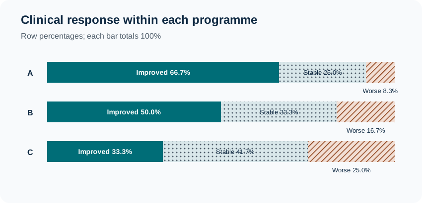
The row percentages are:
- Programme A: 66.7% improved, 25.0% stable, 8.3% worse;
- Programme B: 50.0%, 33.3%, 16.7%;
- Programme C: 33.3%, 41.7%, 25.0%.
Statistical assumptions
Expected counts
For cell :
In this balanced example, the expected counts in every row are 30, 20 and 10.
Traditional rules about expected counts are approximations rather than universal laws. When the table is sparse, consider:
- Fisher’s exact test;
- Monte Carlo simulation;
- an exact conditional method;
- a model suited to the categorical outcome;
- or clinically justified category combination.
Fisher’s exact test
Fisher’s exact test is particularly useful for an independent table when the sample is small or expected counts are sparse. Unlike Pearson’s chi-square test, it does not rely on a large-sample chi-square approximation.
For a table, the test conditions on the observed row and column totals. Under the null hypothesis of no association, it calculates the probabilities of tables with those same margins and evaluates how unusual the observed table is. A two-sided test includes tables considered at least as incompatible with the null hypothesis as the observed table.
Sparse independent 2 × 2 table
simulated dataTable 2. Adverse event by treatment group
| Group | Adverse event | No adverse event | Total |
|---|---|---|---|
| New treatment | 1 | 19 | 20 |
| Usual care | 6 | 14 | 20 |
| Total | 7 | 33 | 40 |
Note: Values are simulated counts from independent participants. The expected adverse-event count is 3.5 in each group, so the Pearson approximation warrants caution.
For this table, the two-sided Fisher’s exact test gives . The data do not provide strong evidence of an association at the 5% significance level, although the observed adverse-event proportion is lower with the new treatment. The estimate is imprecise because only seven events occurred.
The exact enumeration used to calculate the Fisher p-value is performed by R and is not shown here.
Use Fisher’s exact test thoughtfully:
- it is suitable for independent categorical observations, not paired before-and-after data;
- its usual form tests association while conditioning on the margins;
- the direction of a one-sided alternative must be prespecified and scientifically justified;
- exact procedures can be conservative and should not be selected merely because they produce a preferred p-value;
- and exact analysis of larger tables may require substantial computation or Monte Carlo methods.
How the method works
Each cell contributes a non-negative quantity. Cells with larger observed–expected discrepancies contribute more.
Cramer’s V
For an table:
Worked example
Reproducible R analysis
Base R implements Pearson’s chi-square test using chisq.test() and exact conditional analysis using fisher.test() [2].
response_table <- matrix(
  c(
    40, 15, 5,
    30, 20, 10,
    20, 25, 15
  ),
  nrow = 3,
  byrow = TRUE,
  dimnames = list(
    Programme = c("A", "B", "C"),
    Response = c("Improved", "Stable", "Worse")
  )
)

fit <- chisq.test(
  response_table,
  correct = FALSE
)

fit
fit$expected
prop.table(response_table, margin = 1)

n_total <- sum(response_table)
cramers_v <- sqrt(
  unname(fit$statistic) /
    (
      n_total *
        min(nrow(response_table) - 1, ncol(response_table) - 1)
    )
)

output <- data.frame(
  chi_square = unname(fit$statistic),
  df = unname(fit$parameter),
  p_value = fit$p.value,
  cramers_v = cramers_v
)

round(output, 3)


sparse_table <- matrix(
  c(
    1, 19,
    6, 14
  ),
  nrow = 2,
  byrow = TRUE,
  dimnames = list(
    Group = c("New treatment", "Usual care"),
    Outcome = c("Adverse event", "No adverse event")
  )
)

sparse_expected <- chisq.test(
  sparse_table,
  correct = FALSE
)$expected

sparse_fit <- fisher.test(
  sparse_table,
  alternative = "two.sided"
)

sparse_output <- data.frame(
  fisher_p_value = sparse_fit$p.value,
  conditional_odds_ratio = unname(sparse_fit$estimate),
  ci_lower = sparse_fit$conf.int[1],
  ci_upper = sparse_fit$conf.int[2]
)

round(sparse_expected, 1)
round(sparse_output, 3)
R output
	Pearson's Chi-squared test

X-squared = 14.167, df = 4, p-value = 0.006782
Cleaned output
 chi_square df p_value cramers_v
     14.167  4   0.007      0.198
Fisher’s exact test output
 fisher_p_value conditional_odds_ratio ci_lower ci_upper
          0.091                  0.129    0.003    1.246
The odds ratio shown by fisher.test() is a conditional maximum-likelihood estimate. It can differ slightly from the simple cross-product sample odds ratio. The very wide interval reflects the limited information in the sparse table.
Interpreting the output
Presenting the results
Table 2. Clinical response within each programme
| Programme | Improved | Stable | Worse |
|---|---|---|---|
| A | 40 (66.7%) | 15 (25.0%) | 5 (8.3%) |
| B | 30 (50.0%) | 20 (33.3%) | 10 (16.7%) |
| C | 20 (33.3%) | 25 (41.7%) | 15 (25.0%) |
Note: Percentages are row percentages.
Pearson , ; Cramer’s .
Suggested reporting
For the separate sparse example, an appropriate concise report would be:
Cell residuals and follow-up interpretation MMed extension
Pearson residuals are:
They help identify cells contributing to the omnibus statistic.
Formal interpretation of many cell residuals creates another multiplicity problem. Use them descriptively or apply a prespecified adjusted procedure rather than declaring every large residual a separate discovery.
For ordered categories, a trend or ordinal model may be more powerful and interpretable than the general chi-square test when its assumptions match the question [4].
Common mistakes
Knowledge check
What are expected counts?
Answer and reasoning
They are the cell counts predicted under the null hypothesis of independence, calculated from the row total, column total and grand total.
Why are row percentages appropriate in the example?
Answer and reasoning
The question compares the response distribution within each programme. Each row total is therefore the relevant denominator.
Does p = 0.007 identify which specific cells differ?
Answer and reasoning
No. It is an omnibus result. The observed table, residuals and prespecified contrasts are needed to describe the pattern.
Why is Pearson chi-square inappropriate for before-and-after response from the same participants?
Answer and reasoning
The two observations are paired. Pearson’s test assumes independent cell contributions; McNemar or another paired categorical method is required.
What does Cramer's V add?
Answer and reasoning
It provides a standardised summary of overall association strength. It does not replace category-specific percentages or establish causality.
When should Fisher's exact test be considered for an independent 2 × 2 table?
Answer and reasoning
Consider it when the sample or expected counts are too sparse for a reliable Pearson chi-square approximation. The choice should reflect the design and prespecified analysis plan rather than which test gives a preferred p-value.
Why would Fisher's exact test not be appropriate for paired before-and-after binary outcomes?
Answer and reasoning
Fisher’s exact test for a standard table assumes independent observations. Paired binary outcomes require a method based on discordant pairs, such as McNemar’s test or an exact paired-binomial procedure.
Key take-home messages
References
- Pearson K. On the criterion that a given system of deviations from the probable in the case of a correlated system of variables is such that it can reasonably be supposed to have arisen from random sampling. Philos Mag. 1900;50(302):157–175. https://doi.org/10.1080/14786440009463897
- R Core Team. Pearson’s chi-squared test and Fisher’s exact test. R documentation, package stats version 4.6.1. Vienna: R Foundation for Statistical Computing; 2026. https://stat.ethz.ch/R-manual/R-devel/library/stats/html/chisq.test.html
- Agresti A. Categorical data analysis. 3rd ed. Hoboken (NJ): Wiley; 2013.
- Cochran WG. Some methods for strengthening the common chi-square tests. Biometrics. 1954;10(4):417–451. https://doi.org/10.2307/3001616
These notes support learning and research planning and do not replace statistical consultation for a specific study.