Interactions and Effect Modification

Overview

An interaction occurs when the association or treatment effect for one predictor differs according to the level of another predictor.

Effect modification must be defined on a specific scale. A relation can vary on the additive scale but appear constant on a multiplicative scale.

In linear regression, a product term represents departure from additivity of mean effects.

Why this matters

A treatment may work differently according to baseline severity, age or body mass index. Reporting one overall coefficient can conceal clinically important heterogeneity.

Separate subgroup analyses are not an interaction test. The correct analysis directly estimates the difference between subgroup effects [1].

When to use this method

Use an interaction term when effect heterogeneity is prespecified and scientifically plausible.

Avoid indiscriminate searches across many modifiers because false-positive and unstable findings become likely.

Research question and variables

The telemonitoring effect at BMI value $m$ is:

$$\beta_1+\beta_3m$$

Data structure

Interaction variables

simulated data

Variable	Role
Follow-up systolic blood pressure	Numerical outcome
Telemonitoring	Predictor
Centred BMI	Candidate effect modifier
Baseline blood pressure, age, adherence and sex	Adjustment variables

Statistical assumptions

How the method works

Centring BMI makes the telemonitoring main coefficient represent the treatment contrast at mean BMI. Interaction interpretation should prioritise clinically relevant subgroup effects and their uncertainty [2], while retaining a coherent regression specification [3].

The interaction coefficient describes how that contrast changes per one-unit higher BMI.

Main effects in the presence of interaction

Once a product term is included, a main-effect coefficient is conditional on the other interacting variable being zero. For centred BMI, the telemonitoring coefficient is the treatment contrast at mean BMI. For uncentred BMI, it would refer to BMI zero, which is clinically meaningless.

The BMI coefficient represents the BMI slope in the reference treatment group. The BMI slope under telemonitoring is the sum of the BMI main coefficient and the interaction coefficient.

Simple effects and contrasts

Clinically useful interpretation requires calculating treatment effects at meaningful BMI values. These might be prespecified values such as 25 and 30 kg/m² or representative percentiles.

Each simple effect needs its own standard error because it combines two estimated coefficients and their covariance. Merely adding the coefficient confidence-interval endpoints is incorrect.

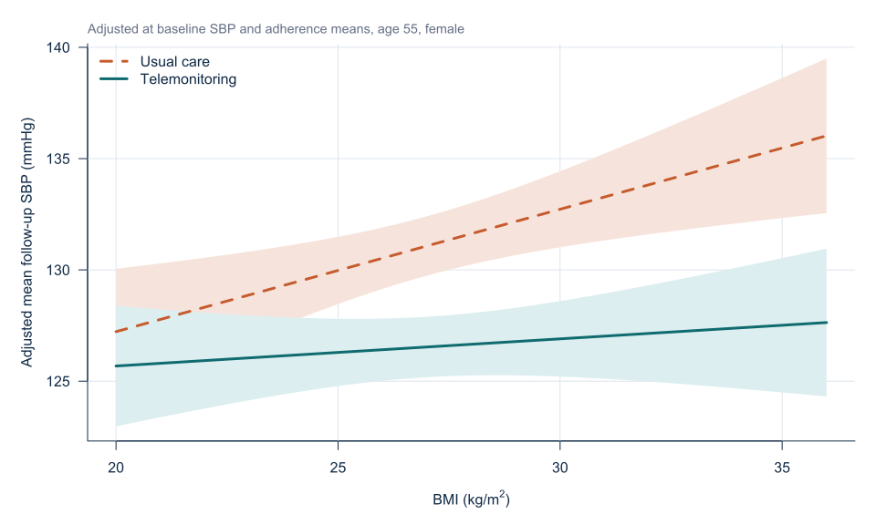
A graph can display fitted treatment lines over BMI with confidence bands. Non-parallel lines visualise interaction, but the plotted range should stay within well-supported joint data regions.

Effect modification versus subgroup analysis

Effect modification is heterogeneity in an effect measure across levels of another variable. Subgroup analysis is the act of estimating effects within subsets. Subgroup estimates can be useful without a formal interaction, but conclusions about differing effects require a direct interaction contrast.

Small subgroups usually yield imprecise estimates. A treatment effect can be statistically significant in a large subgroup and non-significant in a small subgroup even when the point estimates are identical.

Additive and multiplicative scales

In linear regression, the interaction is additive in the outcome mean. In logistic regression, a product term is multiplicative on the odds scale. The presence or absence of interaction can change with the effect scale.

For clinical decisions, absolute risk differences may be more informative than odds-ratio interaction. A model can therefore be used to estimate standardised risks and risk differences across modifier values.

Multiplicity and credibility

Testing many candidate modifiers creates a high chance of apparently positive interactions. Credible effect-modification analysis is strengthened by:

• prespecification;
• a small number of biologically plausible modifiers;
• adequate information across modifier levels;
• consistent direction with prior evidence;
• replication;
• avoidance of cut-point searching.

Exploratory interactions should be labelled clearly and treated as hypotheses for future study.

Continuous modifiers

Dichotomising BMI at a convenient threshold assumes that treatment effects jump abruptly at that point and remain constant within each category. A continuous interaction preserves information but also assumes a linear change in effect. If this is implausible, nonlinear main effects and nonlinear interaction functions may be needed.

Worked example

Reproducible R analysis

make_hypertension_data <- function(n = 180) {
  set.seed(4583)
  i <- seq_len(n)

  data <- data.frame(
    participant_id = sprintf("H%03d", i),
    age = round(runif(n, 30, 80)),
    male = rbinom(n, 1, 0.5),
    bmi = pmin(pmax(round(rnorm(n, 27, 3.5), 1), 18), 40),
    physical_activity = round(runif(n, 2, 7), 1),
    telemonitoring = rbinom(n, 1, 0.5)
  )

  data$adherence <- 4 + runif(n, 0, 5) -
    0.015 * (data$age - 55) + 0.4 * data$telemonitoring
  data$baseline_sbp <- 92 + 0.52 * data$age + 0.85 * data$bmi +
    2.8 * data$male - 1.3 * data$physical_activity + rnorm(n, 0, 4)
  data$followup_sbp <- 58 + 0.47 * data$baseline_sbp +
    0.10 * data$age + 0.52 * data$bmi - 2.0 * data$adherence +
    2.0 * data$male - 4.5 * data$telemonitoring -
    0.55 * data$telemonitoring * (data$bmi - 27) +
    0.006 * (data$age - 55)^2 + rnorm(n, 0, 5)

  data
}

hypertension <- make_hypertension_data()

hypertension$bmi_c <- hypertension$bmi -
  mean(hypertension$bmi)

fit <- lm(
  followup_sbp ~ baseline_sbp + age + adherence +
    male + telemonitoring * bmi_c,
  data = hypertension
)

summary(fit)
confint(fit)

simple_effect <- function(bmi_c_value) {
  b <- coef(fit)
  V <- vcov(fit)

  estimate <- b["telemonitoring"] +
    bmi_c_value * b["telemonitoring:bmi_c"]

  variance <- V["telemonitoring", "telemonitoring"] +
    bmi_c_value^2 *
      V["telemonitoring:bmi_c", "telemonitoring:bmi_c"] +
    2 * bmi_c_value *
      V["telemonitoring", "telemonitoring:bmi_c"]

  se <- sqrt(variance)

  c(
    estimate = estimate,
    lower = estimate - 1.96 * se,
    upper = estimate + 1.96 * se
  )
}

rbind(
  low_bmi = simple_effect(-4),
  mean_bmi = simple_effect(0),
  high_bmi = simple_effect(4)
)

Cleaned R output

Term                         Estimate   95% CI
Telemonitoring at mean BMI    -4.402    -5.918 to -2.886
BMI among usual care           0.550     0.194 to 0.906
Telemonitoring × BMI           -0.428    -0.864 to 0.008

Interpreting the output

Presenting the results

Present the interaction coefficient together with simple effects at clinically meaningful modifier values.

Visualising effect modification

Suggested reporting

Scale dependence MMed extension

For binary outcomes, interaction on the odds-ratio scale can differ from interaction on the risk-difference scale. Clinical effect modification should therefore be evaluated on a scale relevant to decisions [1], [2].

Common mistakes

Knowledge check

What does the interaction coefficient represent?

Answer and reasoning

It is the change in the telemonitoring mean difference per one-unit higher centred BMI.

Why are different subgroup p-values insufficient?

Answer and reasoning

Significance depends on both effect size and precision. A direct difference between effects is required.

Why centre BMI?

Answer and reasoning

It makes the telemonitoring main coefficient interpretable at the mean BMI and reduces unnecessary correlation between product and main terms.

Does statistical interaction prove biological interaction?

Answer and reasoning

No. Statistical interaction is scale- and model-dependent.

Why report simple effects?

Answer and reasoning

They translate the product coefficient into clinically understandable treatment contrasts at relevant modifier values.

Key take-home messages

References

1. VanderWeele TJ, Knol MJ. A tutorial on interaction. Epidemiol Methods. 2014;3(1):33–72. https://doi.org/10.1515/em-2013-0005
2. Kent DM, Rothwell PM, Ioannidis JPA, Altman DG, Hayward RA. Assessing and reporting heterogeneity in treatment effects in clinical trials. Trials. 2010;11:85. https://doi.org/10.1186/1745-6215-11-85
3. Harrell FE Jr. Regression modeling strategies. 2nd ed. Cham: Springer; 2015. https://doi.org/10.1007/978-3-319-19425-7