Kaplan-Meier Survival Analysis

Overview

The Kaplan–Meier estimator is a non-parametric estimator of the survival function under right censoring [1].

It uses the sequence of event times and changing risk sets.

The curve:

• starts at 1;
• drops only when events occur;
• remains flat between events;
• marks censoring times without dropping;
• becomes less precise as the risk set becomes small.

It estimates the probability of remaining event free beyond each time.

Why this matters

A simple observed proportion alive at 24 months can be biased when participants have different follow-up durations.

Kaplan–Meier analysis uses all available event-free follow-up without assuming one parametric survival distribution.

The curve should be accompanied by:

• confidence intervals;
• censoring marks;
• numbers at risk;
• event counts;
• follow-up information.

A curve without its risk table can create false confidence in the unstable tail [2].

When to use this method

Use Kaplan–Meier estimation when:

• the endpoint is time to one event type;
• exact or right-censored times are available;
• delayed entry is handled appropriately;
• independent censoring is plausible.

Do not use one minus the Kaplan–Meier event-free curve as the cumulative incidence of one cause when competing events exist.

Research question and variables

The questions are:

• What proportion is estimated to survive beyond 12, 24 and 36 months?
• What is the median survival in each group?
• How precise are these estimates?

The group comparison itself is developed in the next lecture using the log-rank test and later through Cox regression.

Data structure

Kaplan–Meier inputs

simulated data

Variable	Meaning
overall_time	Months to death or censoring
overall_event	1 = death; 0 = censored
group	Usual care or intervention
id	Participant identifier

One participant contributes one overall-survival record in the simple setting.

Statistical assumptions

How the method works

At event time $t_j$:

• $n_j$ participants are at risk immediately before the time;
• $d_j$ events occur.

The Kaplan–Meier estimator is:

Censoring changes later risk sets but does not create a downward step.

Greenwood standard error

Greenwood’s formula estimates the variance of the Kaplan–Meier curve.

Confidence intervals are commonly constructed on a transformed scale, such as log–log, to remain within 0 and 1.

Worked example

Worked analysis in R

The survival package uses survfit() for Kaplan–Meier curves [3].

make_survival_data <- function(n = 240) {
  id <- seq_len(n)
  group_numeric <- as.integer(id %% 2 == 0)
  age <- 35 + ((7 * id) %% 41)
  stage3 <- as.integer(id %% 3 == 0)

  deterministic_uniform <- function(multiplier) {
    (((id * multiplier) %% 997) + 0.5) / 998
  }

  u_recurrence <- deterministic_uniform(37)
  u_nonrecurrence_death <- deterministic_uniform(73)
  u_postrecurrence_death <- deterministic_uniform(109)
  u_dropout <- deterministic_uniform(149)
  u_dropout_time <- deterministic_uniform(181)

  recurrence_rate <-
    0.035 *
    exp(
      log(0.55) * group_numeric +
      0.025 * (age - 55) +
      0.55 * stage3
    )

  nonrecurrence_death_rate <-
    0.010 *
    exp(
      log(0.85) * group_numeric +
      0.030 * (age - 55) +
      0.40 * stage3
    )

  postrecurrence_death_rate <-
    0.060 *
    exp(
      log(0.85) * group_numeric +
      0.020 * (age - 55) +
      0.25 * stage3
    )

  recurrence_time <-
    -log(u_recurrence) / recurrence_rate

  nonrecurrence_death_time <-
    -log(u_nonrecurrence_death) /
    nonrecurrence_death_rate

  postrecurrence_death_delay <-
    -log(u_postrecurrence_death) /
    postrecurrence_death_rate

  overall_death_time <- pmin(
    nonrecurrence_death_time,
    recurrence_time +
      postrecurrence_death_delay
  )

  dropout_time <- ifelse(
    u_dropout < 0.22,
    12 + 24 * u_dropout_time,
    Inf
  )

  censor_time <- pmin(
    36,
    dropout_time
  )

  overall_time <- pmin(
    overall_death_time,
    censor_time
  )

  overall_event <- as.integer(
    overall_death_time <= censor_time
  )

  competing_time <- pmin(
    recurrence_time,
    nonrecurrence_death_time,
    censor_time
  )

  competing_status <- ifelse(
    recurrence_time <=
      nonrecurrence_death_time &
      recurrence_time <= censor_time,
    1L,
    ifelse(
      nonrecurrence_death_time <
        recurrence_time &
        nonrecurrence_death_time <=
          censor_time,
      2L,
      0L
    )
  )

  data.frame(
    id = id,
    group_numeric = group_numeric,
    group = factor(
      group_numeric,
      levels = c(0, 1),
      labels = c(
        "Usual care",
        "Intervention"
      )
    ),
    age = age,
    stage3 = stage3,
    stage = factor(
      stage3,
      levels = c(0, 1),
      labels = c("Stage II", "Stage III")
    ),
    overall_time = overall_time,
    overall_event = overall_event,
    competing_time = competing_time,
    competing_status = competing_status
  )
}

survival_data <- make_survival_data()

library(survival)

km_fit <- survfit(
  Surv(
    overall_time,
    overall_event
  ) ~ group,
  data = survival_data,
  conf.type = "log-log"
)

km_fit

summary(
  km_fit,
  times = c(12, 24, 36),
  extend = TRUE
)

quantile(
  km_fit,
  probs = 0.5
)

plot(
  km_fit,
  xlab = "Months from treatment allocation",
  ylab = "Overall-survival probability",
  mark.time = TRUE,
  conf.int = TRUE,
  xlim = c(0, 36)
)

legend(
  "bottomleft",
  legend = levels(survival_data$group),
  lty = 1:2
)

Selected analysis output

Group          N   Deaths   Median   S(12)   S(24)   S(36)
Usual care   120      80     22.5    0.717   0.455   0.301
Intervention 120      64     28.0    0.842   0.595   0.433

The displayed estimates are derived from the simulated dataset and can be recalculated using the accompanying R code.

Visualising Kaplan–Meier survival

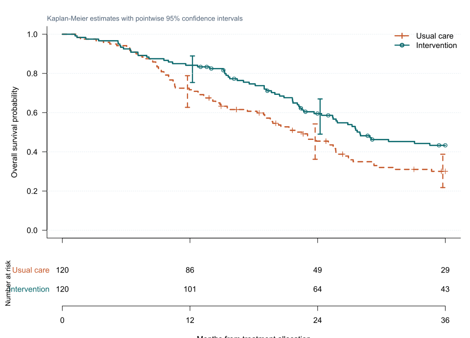
The curve should use:

• a probability scale from 0 to 1;
• a clearly labelled time unit;
• censoring marks;
• a number-at-risk table;
• groups distinguishable without colour alone;
• a sensible end point based on remaining information.

Reading censoring marks

A censoring mark indicates the last known event-free time.

It does not cause the curve to fall.

A dense group of early censoring marks can signal incomplete follow-up or a different censoring pattern between groups.

Median survival

Median survival can be:

• estimated;
• not reached;
• poorly estimated.

If the curve never falls to 0.50, report:

Median survival was not reached during the observed follow-up.

Do not substitute the largest follow-up time.

Landmark survival

Survival at a prespecified landmark can be more interpretable than the median.

Report:

• landmark;
• estimate;
• confidence interval;
• number at risk near that time.

Avoid selecting the landmark after examining where curves appear most separated.

The unstable tail

At late times:

• few participants remain at risk;
• censoring accumulates;
• confidence intervals widen;
• a single event can cause a large step.

The number-at-risk table reveals this loss of information.

The curve should not be extended visually beyond meaningful follow-up merely because the last censored participant remains.

Interpreting the output

Presenting the results

Suggested reporting

Report the time origin, event count, censoring rule, median with CI when estimable, landmark survival with CI, censor marks and numbers at risk.

Good-practice recommendations caution against truncated axes, omitted risk tables and overinterpretation of sparse curve tails [2], [4].

Common mistakes

Knowledge check

When does a Kaplan–Meier curve drop?

Answer and reasoning

Only when one or more events occur.

What does a censoring mark mean?

Answer and reasoning

The participant was event free until that time, after which the event time is unknown.

How is median survival defined?

Answer and reasoning

It is the earliest time at which the estimated survival probability reaches or falls below 0.50.

Why include numbers at risk?

Answer and reasoning

They show how much information supports each part of the curve, especially the tail.

Does a visible gap between curves prove a treatment effect?

Answer and reasoning

No. Formal comparison, uncertainty, design validity and assumptions are still required.

Key take-home messages

References

1. Kaplan EL, Meier P. Nonparametric estimation from incomplete observations. J Am Stat Assoc. 1958;53(282):457–481. https://doi.org/10.1080/01621459.1958.10501452
2. Pocock SJ, Clayton TC, Altman DG. Survival plots of time-to-event outcomes in clinical trials: good practice and pitfalls. Lancet. 2002;359(9318):1686–1689. https://doi.org/10.1016/S0140-6736(02)08594-X
3. Therneau TM. A package for survival analysis in R. R package survival version 3.8-9. 2026. https://CRAN.R-project.org/package=survival
4. Morris TP, Jarvis CI, Cragg W, Phillips PPJ, Choodari-Oskooei B, Sydes MR. Proposals on Kaplan–Meier plots in medical research and a survey of stakeholder views. Res Synth Methods. 2019;10(4):617–626. https://doi.org/10.1002/jrsm.1351