
Part 7 · Module 4
Paired Categorical Data
Learn how to analyse paired binary outcomes using discordant pairs, McNemar's test, paired risk difference and reproducible R output.
Learning outcomes
After completing this lecture, you should be able to:
- Recognise paired binary outcomes and construct the paired two-by-two table.
- Explain why McNemar's test uses discordant pairs.
- Calculate and interpret a paired proportion difference and confidence interval.
- Distinguish asymptotic and exact McNemar procedures.
- Explain why an ordinary independent chi-square test is inappropriate.
- Use reproducible R code to perform and report a paired categorical analysis.
Overview
Paired categorical data arise when two binary measurements are linked within the same analytical unit or matched pair.
Examples include:
- disease status before and after an intervention;
- two diagnostic tests applied to the same participant;
- matched case–control exposure status;
- two raters classifying the same specimen;
- presence or absence of a symptom at two visits.
For two paired binary outcomes, McNemar’s test evaluates whether the marginal proportions are equal by comparing the two types of discordant pair [1].
The method is not an ordinary chi-square test of independence. Agreement and marginal change are different questions.
Why this matters
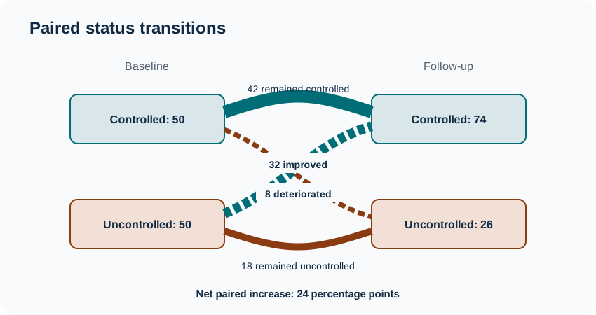
Suppose 100 participants are classified as controlled or not controlled at baseline and follow-up.
Participants who are:
- not controlled at both times;
- controlled at both times
show agreement but do not indicate the direction of change.
The directional information comes from:
- not controlled → controlled;
- controlled → not controlled.
McNemar’s test compares these discordant counts.
A large number of concordant pairs can produce high agreement while the marginal proportion still changes. Conversely, equal marginal proportions can coexist with poor individual agreement.
When to use this method
Use McNemar’s test when:
- the outcome is binary at both measurements;
- observations are paired correctly;
- pairs are independent of other pairs;
- the question concerns equality of the two marginal proportions;
- and discordant counts support the chosen asymptotic or exact method.
Do not use it to assess:
- agreement between classifications;
- two independent groups;
- more than two repeated occasions;
- multi-category paired outcomes without an extension;
- or causal intervention effects without an appropriate comparison design.
Research question and variables
Define positive as controlled blood pressure.
The baseline controlled proportion is:
The follow-up controlled proportion is:
The paired risk difference is:
The McNemar null is:
Data structure
Paired binary table
simulated dataTable 1. Blood-pressure control at baseline and follow-up
| Baseline status | Follow-up uncontrolled | Follow-up controlled | Total |
|---|---|---|---|
| Uncontrolled | 18 | 32 | 50 |
| Controlled | 8 | 42 | 50 |
| Total | 26 | 74 | 100 |
Note: The discordant cells are 32 and 8. Counts are simulated.
The table orientation must be stated. Reversing rows or columns reverses the paired-difference sign but not the two-sided test.
Statistical assumptions
Participants missing either measurement do not contribute to the complete-pair McNemar table. Excluding them may bias the result if completeness is related to outcome change.
How the method works
Without continuity correction, the asymptotic statistic is:
For small discordant totals, an exact conditional test treats as a binomial count among discordant pairs under probability 0.5.
Paired proportion difference
The estimated change is:
An approximate standard error is:
This interval should be interpreted cautiously when discordant counts are small. Improved paired-binomial interval methods are available [2].
Worked example
Reproducible R analysis
Base R implements McNemar’s test using mcnemar.test() [3].
paired_table <- matrix(
  c(
    18, 32,
    8, 42
  ),
  nrow = 2,
  byrow = TRUE,
  dimnames = list(
    Baseline = c("Uncontrolled", "Controlled"),
    Followup = c("Uncontrolled", "Controlled")
  )
)

fit <- mcnemar.test(
  paired_table,
  correct = FALSE
)

b <- paired_table["Uncontrolled", "Controlled"]
c <- paired_table["Controlled", "Uncontrolled"]
n <- sum(paired_table)

baseline_controlled <- sum(paired_table["Controlled", ]) / n
followup_controlled <- sum(paired_table[, "Controlled"]) / n
paired_difference <- (b - c) / n

paired_se <- sqrt(
  (
    b + c - (b - c)^2 / n
  ) / n^2
)

paired_ci <- paired_difference + c(-1, 1) * 1.96 * paired_se

exact_fit <- binom.test(
  x = b,
  n = b + c,
  p = 0.5,
  alternative = "two.sided"
)

output <- data.frame(
  baseline_percent = 100 * baseline_controlled,
  followup_percent = 100 * followup_controlled,
  difference_pp = 100 * paired_difference,
  ci_lower_pp = 100 * paired_ci[1],
  ci_upper_pp = 100 * paired_ci[2],
  mcnemar_chi_square = unname(fit$statistic),
  asymptotic_p = fit$p.value,
  exact_p = exact_fit$p.value
)

round(output, 3)
R output
	McNemar's Chi-squared test

McNemar's chi-squared = 14.4, df = 1, p-value = 0.0001478
Cleaned output
 baseline_percent followup_percent difference_pp ci_lower_pp ci_upper_pp mcnemar_chi_square asymptotic_p exact_p
             50.0             74.0          24.0      12.531      35.469               14.4     0.000148 0.000182
Report both p-values as $p<0.001$, not p=0.000.
Interpreting the output
Presenting the results
Table 2. Paired change in blood-pressure control
| Measure | Estimate |
|---|---|
| Baseline controlled | 50 / 100 (50.0%) |
| Follow-up controlled | 74 / 100 (74.0%) |
| Paired difference | 24.0 percentage points |
| 95% CI | 12.5 to 35.5 percentage points |
McNemar , ; exact discordant-pair .
Suggested reporting
Paired multi-category outcomes MMed extension
For more than two paired nominal categories, categorical-data extensions are required [4]:
- Stuart–Maxwell test of marginal homogeneity;
- Bowker test of symmetry;
- multinomial marginal models.
For repeated binary outcomes at more than two times, consider:
- generalised estimating equations;
- mixed-effects logistic regression;
- transition models.
These methods answer different marginal or subject-specific questions.
Common mistakes
Knowledge check
Which cells determine McNemar's test?
Answer and reasoning
The two discordant cells: participants changing from uncontrolled to controlled and those changing from controlled to uncontrolled.
Why do the 18 and 42 concordant cells not determine the direction of change?
Answer and reasoning
They represent participants whose status stayed the same. They contribute to marginal prevalence but not to the imbalance between the two change directions.
Does McNemar's test assess agreement?
Answer and reasoning
No. It tests equality of paired marginal proportions. Agreement requires measures such as observed agreement and kappa, interpreted in a separate framework.
Why might an exact McNemar test be preferred?
Answer and reasoning
When the total number of discordant pairs is small, the chi-square approximation may be inaccurate. The exact binomial procedure conditions on the discordant total.
Can this before-and-after result establish programme effectiveness?
Answer and reasoning
No. Without an appropriate control group, secular changes, regression to the mean and co-interventions may explain part of the change.
Key take-home messages
References
- McNemar Q. Note on the sampling error of the difference between correlated proportions or percentages. Psychometrika. 1947;12(2):153–157. https://doi.org/10.1007/BF02295996
- Newcombe RG. Improved confidence intervals for the difference between binomial proportions based on paired data. Stat Med. 1998;17(22):2635–2650. https://doi.org/10.1002/(SICI)1097-0258(19981130)17:22%3C2635::AID-SIM954%3E3.0.CO;2-C
- R Core Team. McNemar’s chi-squared test. R documentation, package stats version 4.6.1. Vienna: R Foundation for Statistical Computing; 2026. https://stat.ethz.ch/R-manual/R-devel/library/stats/html/mcnemar.test.html
- Agresti A. Categorical data analysis. 3rd ed. Hoboken (NJ): Wiley; 2013.
These notes support learning and research planning and do not replace statistical consultation for a specific study.