
Part 10 · Module 4
Cox Proportional Hazards Regression
Learn how Cox regression estimates adjusted hazard ratios, handles censored follow-up, checks proportional hazards and produces adjusted survival curves.
Learning outcomes
After completing this lecture, you should be able to:
- Explain the Cox proportional-hazards model and partial likelihood.
- Interpret adjusted hazard ratios for binary and continuous predictors.
- Distinguish hazard ratios from risk ratios and survival probabilities.
- Assess proportional hazards using Schoenfeld residuals and time interactions.
- Recognise non-linearity, influential observations, ties and time-dependent covariates.
- Use reproducible R code to fit, diagnose and report a Cox model.
Overview
Cox proportional-hazards regression relates predictors to the event hazard while leaving the baseline hazard unspecified [1].
The model is:
where:
- is the baseline hazard;
- contains log hazard ratios.
Exponentiating a coefficient gives a hazard ratio conditional on the other included predictors.
Why this matters
The Cox model can:
- adjust for prognostic factors;
- estimate treatment or exposure hazard ratios;
- model continuous predictors;
- incorporate strata;
- include time-dependent covariates;
- generate adjusted survival curves.
A hazard ratio is not:
- a risk ratio;
- a ratio of median survival;
- a probability;
- a constant difference in survival probability.
Its interpretation depends critically on proportional hazards and the selected covariates.
When to use this method
Use Cox regression when:
- the endpoint is a censored time to event;
- adjusted relative hazard is scientifically meaningful;
- the proportional-hazards structure is reasonable or extended appropriately;
- covariate functional forms are suitable;
- censoring assumptions are plausible.
Use alternative models or estimands when hazard ratios are difficult to interpret or strongly time varying.
Research question and variables
The model is:
The intervention hazard ratio is .
Data structure
Cox-model variables
simulated data| Variable | Coding |
|---|---|
overall_time | Months to death or censoring |
overall_event | 1 = death; 0 = censored |
group | Usual care reference |
age10 | Age difference per ten years from 55 |
stage | Stage II reference; stage III comparison |
Reference coding and scaling must be stated in the report.
Statistical assumptions
How the method works
Partial likelihood
At each event time, the model compares the predictor values of the participant experiencing the event with those in the risk set.
The baseline hazard cancels from the partial likelihood, allowing to be estimated without specifying a parametric hazard shape.
Tied events
When several events share the same recorded time, methods include:
- Efron;
- Breslow;
- exact partial likelihood.
Efron’s method is a common default for ordinary Cox regression.
Baseline survival
After estimating coefficients, the baseline cumulative hazard can be estimated and used to generate survival curves for defined covariate profiles.
Worked example
Worked analysis in R
The survival package implements Cox regression using coxph() and proportional-hazards diagnostics using cox.zph() [2].
make_survival_data <- function(n = 240) {
  id <- seq_len(n)
  group_numeric <- as.integer(id %% 2 == 0)
  age <- 35 + ((7 * id) %% 41)
  stage3 <- as.integer(id %% 3 == 0)

  deterministic_uniform <- function(multiplier) {
    (((id * multiplier) %% 997) + 0.5) / 998
  }

  u_recurrence <- deterministic_uniform(37)
  u_nonrecurrence_death <- deterministic_uniform(73)
  u_postrecurrence_death <- deterministic_uniform(109)
  u_dropout <- deterministic_uniform(149)
  u_dropout_time <- deterministic_uniform(181)

  recurrence_rate <-
    0.035 *
    exp(
      log(0.55) * group_numeric +
      0.025 * (age - 55) +
      0.55 * stage3
    )

  nonrecurrence_death_rate <-
    0.010 *
    exp(
      log(0.85) * group_numeric +
      0.030 * (age - 55) +
      0.40 * stage3
    )

  postrecurrence_death_rate <-
    0.060 *
    exp(
      log(0.85) * group_numeric +
      0.020 * (age - 55) +
      0.25 * stage3
    )

  recurrence_time <-
    -log(u_recurrence) / recurrence_rate

  nonrecurrence_death_time <-
    -log(u_nonrecurrence_death) /
    nonrecurrence_death_rate

  postrecurrence_death_delay <-
    -log(u_postrecurrence_death) /
    postrecurrence_death_rate

  overall_death_time <- pmin(
    nonrecurrence_death_time,
    recurrence_time +
      postrecurrence_death_delay
  )

  dropout_time <- ifelse(
    u_dropout < 0.22,
    12 + 24 * u_dropout_time,
    Inf
  )

  censor_time <- pmin(
    36,
    dropout_time
  )

  overall_time <- pmin(
    overall_death_time,
    censor_time
  )

  overall_event <- as.integer(
    overall_death_time <= censor_time
  )

  competing_time <- pmin(
    recurrence_time,
    nonrecurrence_death_time,
    censor_time
  )

  competing_status <- ifelse(
    recurrence_time <=
      nonrecurrence_death_time &
      recurrence_time <= censor_time,
    1L,
    ifelse(
      nonrecurrence_death_time <
        recurrence_time &
        nonrecurrence_death_time <=
          censor_time,
      2L,
      0L
    )
  )

  data.frame(
    id = id,
    group_numeric = group_numeric,
    group = factor(
      group_numeric,
      levels = c(0, 1),
      labels = c(
        "Usual care",
        "Intervention"
      )
    ),
    age = age,
    stage3 = stage3,
    stage = factor(
      stage3,
      levels = c(0, 1),
      labels = c("Stage II", "Stage III")
    ),
    overall_time = overall_time,
    overall_event = overall_event,
    competing_time = competing_time,
    competing_status = competing_status
  )
}

survival_data <- make_survival_data()

library(survival)

survival_data$age10 <-
  (survival_data$age - 55) / 10

cox_fit <- coxph(
  Surv(
    overall_time,
    overall_event
  ) ~ group + age10 + stage,
  data = survival_data,
  ties = "efron",
  x = TRUE,
  model = TRUE
)

summary(cox_fit)

exp(
  cbind(
    hazard_ratio = coef(cox_fit),
    confint(cox_fit)
  )
)

ph_test <- cox.zph(
  cox_fit,
  transform = "km"
)

ph_test
plot(ph_test)

reference_profiles <- data.frame(
  group = factor(
    c(
      "Usual care",
      "Intervention"
    ),
    levels = levels(
      survival_data$group
    )
  ),
  age10 = 0,
  stage = factor(
    "Stage II",
    levels = levels(
      survival_data$stage
    )
  )
)

adjusted_curves <- survfit(
  cox_fit,
  newdata = reference_profiles
)

plot(
  adjusted_curves,
  xlab = "Months from treatment allocation",
  ylab = "Adjusted survival probability",
  xlim = c(0, 36)
)
Selected coefficient output
Predictor                    Adjusted HR   95% CI          p-value
Intervention                    0.654     0.470 to 0.909   0.011
Age per 10 years                1.432     1.244 to 1.649  <0.001
Stage III versus stage II       1.705     1.218 to 2.386   0.002
The Schoenfeld-residual assessment for this simulated example shows no material time trend for intervention, age or stage. This diagnostic should be interpreted alongside the plotted residual pattern and the clinical plausibility of a constant hazard ratio.
Visualising adjusted survival
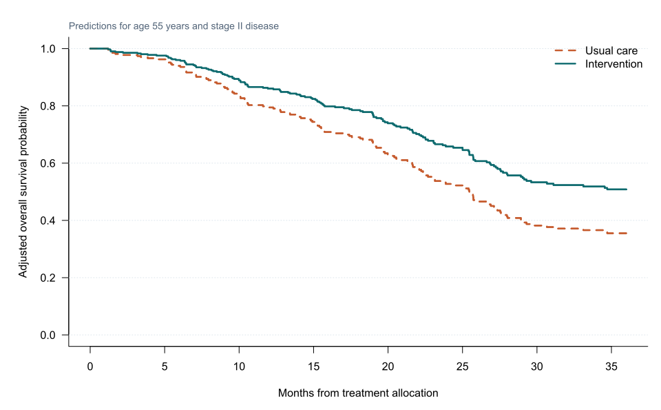
For age 55 and stage II, the approximate adjusted survival probabilities are:
| Group | 12 months | 24 months | 36 months |
|---|---|---|---|
| Usual care | 79.4% | 52.7% | 35.5% |
| Intervention | 86.0% | 65.8% | 50.8% |
These profile-specific curves are not automatically population-standardised treatment effects.
Proportional hazards
The proportional-hazards assumption means:
It does not require the baseline hazard to be constant.
Schoenfeld residuals
Schoenfeld residuals are defined at event times and can be examined for a systematic relationship with time [3].
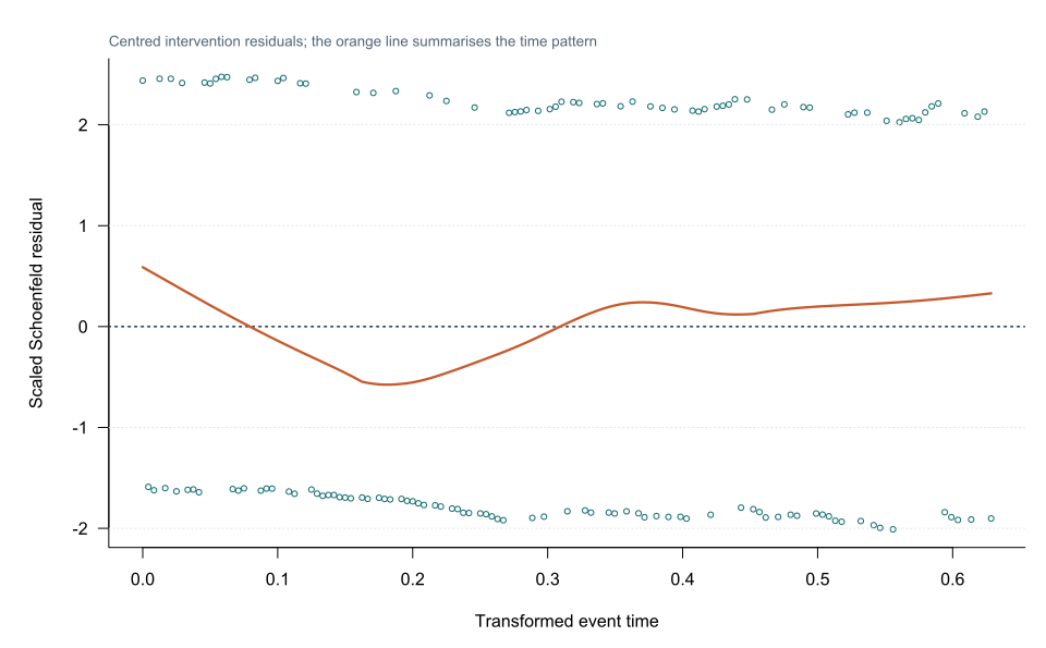
A non-significant cox.zph() test does not prove proportionality.
Examine:
- plots;
- clinical plausibility;
- follow-up support;
- power to detect time variation.
Non-proportional hazards
Possible responses include:
- treatment-by-time interaction;
- piecewise hazard ratios;
- stratification for nuisance predictors;
- flexible parametric survival models;
- landmark survival differences;
- restricted mean survival time.
One average hazard ratio can be difficult to interpret when effects vary or curves cross.
Continuous predictors
A linear age coefficient assumes a constant log-hazard increase per ten years.
Assess non-linearity using:
- residual plots;
- splines;
- fractional polynomials;
- clinically justified transformations.
Categorising age is not a reliable diagnostic solution.
Time-dependent covariates
A predictor such as treatment response may change over follow-up.
Time-dependent covariates require start–stop data:
Surv(start, stop, event)Using a future response value at baseline creates immortal-time and temporal-order bias.
Influential observations
Diagnostics include:
- deviance residuals;
- martingale residuals;
- score residuals;
- dfbeta values.
An influential participant should trigger data verification and sensitivity analysis rather than automatic exclusion.
Interpreting the output
Presenting the results
Suggested reporting
Report event count, candidate predictors, units, reference groups, ties method, proportional-hazards assessment, adjusted HRs with CIs, and adjusted survival probabilities where clinically useful.
The Cox model and Schoenfeld-residual extensions should be interpreted using the complete model and time scale rather than a coefficient table alone [1], [3], [4]. Extended Cox-model implementation and interpretation are described by Therneau and Grambsch [5].
Common mistakes
Knowledge check
What does HR 0.654 mean?
Answer and reasoning
The intervention death hazard is estimated to be 0.654 times the usual-care hazard at a given time among participants still at risk and with the same modelled age and stage.
Does proportional hazards mean the hazard is constant?
Answer and reasoning
No. It means the hazard ratio between profiles is constant; the baseline hazard may change freely over time.
Why use Schoenfeld residuals?
Answer and reasoning
They help assess whether coefficient effects show a systematic trend with event time.
When is ML partial likelihood used in Cox regression?
Answer and reasoning
The Cox coefficients are estimated using partial likelihood based on risk sets at event times.
How should non-proportional treatment effects be reported?
Answer and reasoning
Use time-varying effects or alternative summaries such as landmark survival or restricted mean survival time, with prespecified interpretation.
Key take-home messages
References
- Cox DR. Regression models and life-tables. J R Stat Soc Series B Stat Methodol. 1972;34(2):187–220. https://doi.org/10.1111/j.2517-6161.1972.tb00899.x
- Therneau TM. A package for survival analysis in R. R package survival version 3.8-9. 2026. https://CRAN.R-project.org/package=survival
- Schoenfeld D. Partial residuals for the proportional hazards regression model. Biometrika. 1982;69(1):239–241. https://doi.org/10.1093/biomet/69.1.239
- Grambsch PM, Therneau TM. Proportional hazards tests and diagnostics based on weighted residuals. Biometrika. 1994;81(3):515–526. https://doi.org/10.1093/biomet/81.3.515
- Therneau TM, Grambsch PM. Modeling survival data: extending the Cox model. New York: Springer; 2000. https://doi.org/10.1007/978-1-4757-3294-8
These notes support learning and research planning and do not replace statistical consultation for a specific study.