
Part 6 · Module 3
Independent-Samples t-Test
Learn how to compare two independent population means using Welch's t-test, confidence intervals, effect estimates and reproducible R output.
Learning outcomes
After completing this lecture, you should be able to:
- Identify when two groups are statistically independent.
- State the estimand and hypotheses for comparing two population means.
- Explain why Welch's t-test is generally preferred to the equal-variance pooled t-test.
- Calculate and interpret the mean difference, standard error, confidence interval, t-statistic and p-value.
- Use reproducible R code to perform and verify an independent-samples t-test.
- Report the comparison using clinical units, group summaries and an effect estimate.
Overview
The independent-samples t-test compares the means of a numerical outcome between two independent groups.
Examples include comparing:
- mean systolic blood pressure between two treatment groups;
- mean haemoglobin concentration between exposed and unexposed participants;
- mean functional score between two rehabilitation programmes; and
- mean hospital stay between two independently sampled patient groups.
The primary effect estimate is the difference between population means. The test should therefore be reported with the group means, mean difference and 95% confidence interval rather than a p-value alone.
Two versions are commonly encountered:
- the pooled Student t-test, which assumes equal population variances;
- Welch’s t-test, which allows unequal variances and uses adjusted degrees of freedom.
Welch’s procedure is generally a safer default for two independent groups because it performs well when variances or sample sizes differ and has little disadvantage when variances are equal [1], [2]. The base-R t.test() function uses Welch’s modification by default when var.equal = FALSE [3].
Why this matters
Researchers sometimes decide between pooled and Welch tests using a preliminary variance test. This two-stage strategy is not recommended because the variance test has its own error and makes the final procedure data-dependent.
Another common mistake is to perform a one-sample or paired test because both groups were measured at the same calendar time. Independence concerns whether observations belong to different analytical units, not whether measurements were collected simultaneously.
The important questions are:
- Are the participants in one group different from those in the other?
- Is there one outcome value per participant?
- Is the arithmetic mean the intended estimand?
- Does the analysis need adjustment for baseline or confounders?
If covariate adjustment is required, linear regression or analysis of covariance is usually preferable to a simple t-test.
When to use this method
Use an independent-samples t-test when:
- the outcome is numerical;
- exactly two independent groups are compared;
- each participant contributes one outcome value;
- the population mean is the target;
- no covariate adjustment is required for the primary analysis; and
- the sampling and distributional assumptions are sufficiently reasonable.
Do not use it when:
- the same participants are measured twice;
- participants are matched into pairs;
- repeated observations are nested within participants;
- participants are clustered within clinics or schools without adjustment;
- more than two groups form the primary comparison;
- or baseline adjustment is required in a randomised trial.
Research question and variables
The population parameter is:
where:
- is the telemonitoring population mean;
- is the usual-care population mean.
The two-sided hypotheses are:
Negative values favour telemonitoring because lower systolic blood pressure is desirable in this scenario.
Data structure
Simulated independent-group data
simulated dataTable 1. First four records per group
| participant_id | group | sbp_week12 |
|---|---|---|
| T001 | Telemonitoring | 138 |
| T002 | Telemonitoring | 138 |
| T003 | Telemonitoring | 130 |
| T004 | Telemonitoring | 139 |
| U001 | Usual care | 129 |
| U002 | Usual care | 141 |
| U003 | Usual care | 137 |
| U004 | Usual care | 138 |
Note: One row represents one participant. The complete simulated dataset contains 60 participants.
The grouping variable should be stored as a factor with clear labels. The outcome should retain its clinical unit.
Statistical assumptions
Welch’s test does not require equal population variances. A rank-based method is not an automatic replacement for a mean comparison because it targets a different contrast [4].
It does not correct:
- confounding in an observational study;
- baseline imbalance when an adjusted trial analysis is required;
- cluster dependence;
- informative missingness;
- or poor outcome measurement.
How the method works
The estimated mean difference is:
The Welch standard error is:
The test statistic is:
Welch–Satterthwaite degrees of freedom are calculated from the two variance contributions and can be non-integer [1].
Worked example
Reproducible R analysis
trial <- data.frame(
  participant_id = sprintf("%s%03d", rep(c("T", "U"), each = 30), 1:30),
  group = factor(
    rep(c("Telemonitoring", "Usual care"), each = 30),
    levels = c("Telemonitoring", "Usual care")
  ),
  sbp_week12 = c(
    138, 138, 130, 139, 159, 136, 108, 138, 149, 139,
    127, 126, 130, 122, 132, 138, 121, 134, 137, 126,
    109, 125, 141, 108, 99, 136, 121, 139, 148, 145,
    129, 141, 137, 138, 140, 133, 121, 137, 129, 156,
    137, 158, 143, 152, 138, 130, 146, 153, 132, 146,
    133, 141, 120, 155, 146, 151, 141, 127, 153, 117
  )
)

group_summary <- aggregate(
  sbp_week12 ~ group,
  data = trial,
  FUN = function(x) c(n = length(x), mean = mean(x), sd = sd(x))
)

fit <- t.test(
  sbp_week12 ~ group,
  data = trial,
  var.equal = FALSE,
  alternative = "two.sided",
  conf.level = 0.95
)

fit
R console output
	Welch Two Sample t-test

data:  sbp_week12 by group
t = -2.5600, df = 56.045, p-value = 0.01319
alternative hypothesis: true difference in means between group Telemonitoring and group Usual care is not equal to 0
95 percent confidence interval:
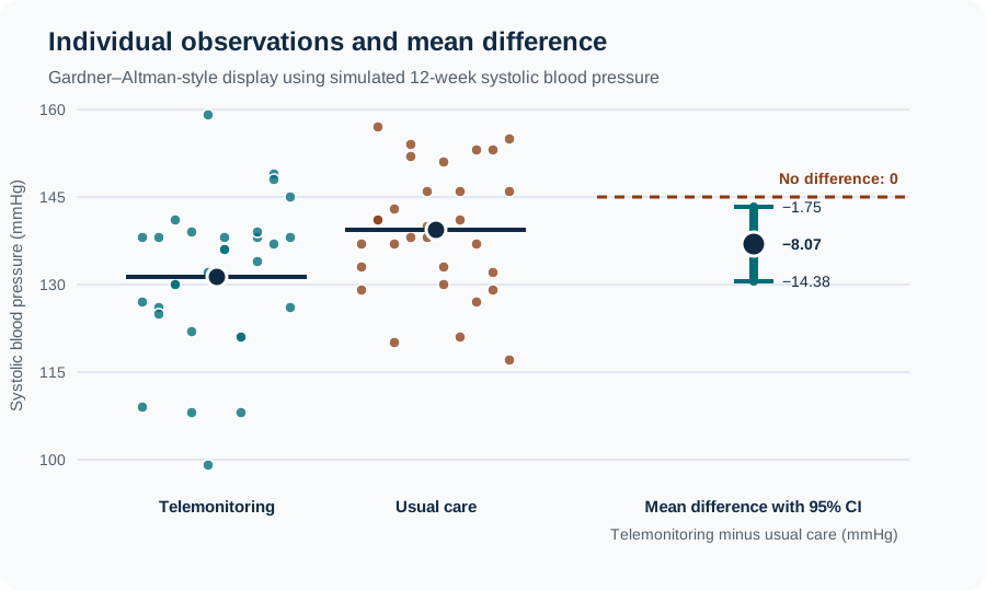
 -14.37894  -1.75439
sample estimates:
mean in group Telemonitoring     mean in group Usual care
                     131.2667                      139.3333
Cleaned output code
x <- trial$sbp_week12[trial$group == "Telemonitoring"]
y <- trial$sbp_week12[trial$group == "Usual care"]

sp <- sqrt(
  ((length(x) - 1) * var(x) + (length(y) - 1) * var(y)) /
    (length(x) + length(y) - 2)
)

cohen_d <- (mean(x) - mean(y)) / sp
hedges_correction <- 1 - 3 / (4 * (length(x) + length(y)) - 9)
hedges_g <- hedges_correction * cohen_d

result <- data.frame(
  mean_telemonitoring = round(mean(x), 2),
  sd_telemonitoring = round(sd(x), 2),
  mean_usual_care = round(mean(y), 2),
  sd_usual_care = round(sd(y), 2),
  mean_difference = round(unname(diff(rev(fit$estimate))), 2),
  ci_lower = round(fit$conf.int[1], 2),
  ci_upper = round(fit$conf.int[2], 2),
  t = round(unname(fit$statistic), 3),
  df = round(unname(fit$parameter), 2),
  p_value = round(fit$p.value, 3),
  hedges_g = round(hedges_g, 2)
)

print(result, row.names = FALSE)
Cleaned R output
 mean_telemonitoring sd_telemonitoring mean_usual_care sd_usual_care mean_difference ci_lower ci_upper      t    df p_value hedges_g
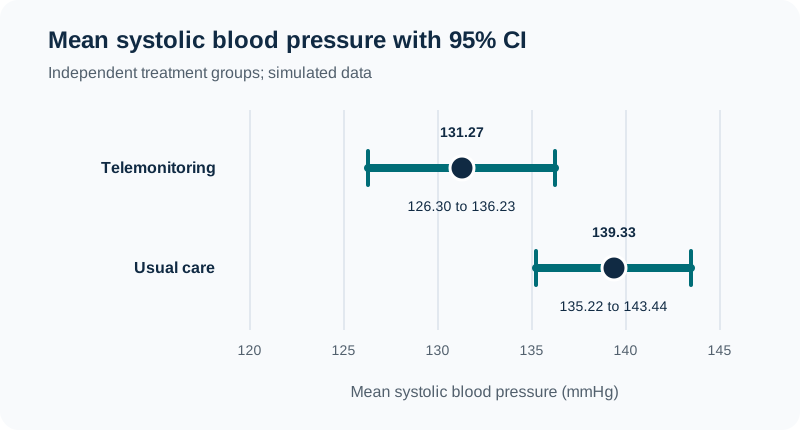
               131.27             13.29          139.33         11.01           -8.07   -14.38    -1.75 -2.560 56.05   0.013    -0.65
Interpreting the output
Presenting the results
| Group | n | Mean (SD), mmHg |
|---|---|---|
| Telemonitoring | 30 | 131.3 (13.3) |
| Usual care | 30 | 139.3 (11.0) |
Mean difference −8.1 mmHg (95% CI −14.4 to −1.8); Welch , .
Visualising the results
Suggested reporting
Why baseline-adjusted analysis may be preferable in a trial MMed extension
When baseline outcome is measured, analysis of covariance commonly estimates the treatment effect more efficiently than an unadjusted follow-up comparison or a comparison of change scores.
The adjusted model should be prespecified and should include treatment allocation and baseline outcome. BIO-P06-M07 develops this approach.
Common mistakes
Knowledge check
Why are these groups independent?
Answer and reasoning
Each participant belongs to only one group and contributes one primary outcome. No participant is paired or repeated across groups.
Why is Welch's test preferred as the default?
Answer and reasoning
It allows unequal population variances and adjusts the degrees of freedom. It remains valid and efficient in many settings where the pooled test’s equal-variance assumption is questionable.
What does the mean difference of −8.1 mmHg represent?
Answer and reasoning
It is the estimated telemonitoring minus usual-care difference in population mean 12-week systolic blood pressure. Negative values indicate a lower mean with telemonitoring.
Does p = 0.013 mean there is a 1.3% probability that the groups have equal means?
Answer and reasoning
No. It is the probability, under the null model and assumptions, of obtaining a test statistic at least as extreme as observed. It is not the probability that the null is true.
When should linear regression replace the simple test?
Answer and reasoning
Use regression when covariate adjustment, stratification variables, interactions, clustering or another model-based effect estimate is required.
Key take-home messages
References
- Welch BL. The generalization of Student’s problem when several different population variances are involved. Biometrika. 1947;34(1–2):28–35. https://doi.org/10.1093/biomet/34.1-2.28
- Delacre M, Lakens D, Leys C. Why psychologists should by default use Welch’s t-test instead of Student’s t-test. Int Rev Soc Psychol. 2017;30(1):92–101. https://doi.org/10.5334/irsp.82
- R Core Team. Student’s t-test. R documentation, package stats version 4.6.1. Vienna: R Foundation for Statistical Computing; 2026. https://search.r-project.org/R/refmans/stats/html/t.test.html
- Altman DG, Bland JM. Parametric v non-parametric methods for data analysis. BMJ. 2009;338:a3167. https://doi.org/10.1136/bmj.a3167
- Lakens D. Calculating and reporting effect sizes to facilitate cumulative science: a practical primer for t-tests and ANOVAs. Front Psychol. 2013;4:863. https://doi.org/10.3389/fpsyg.2013.00863
These notes support learning and research planning and do not replace statistical consultation for a specific study.