Introduction to Time-to-Event Data

Overview

Time-to-event analysis studies both:

• whether an event occurs;
• when it occurs.

Examples include time from:

• randomisation to death;
• surgery to recurrence;
• diagnosis to treatment failure;
• admission to discharge;
• treatment initiation to adverse event;
• birth to disease onset.

Some participants do not experience the event during observation. Their exact event times are unknown, but their observed follow-up still provides information. Survival methods incorporate these censored observations rather than excluding them.

Downloadable simulated dataset

The shared Part 10 dataset is entirely simulated and contains no real patient information. Download the participant-level CSV, read the data dictionary and usage notes, or use the standalone R regeneration script.

The latent-time columns document the simulation mechanism. They represent event times that would not all be observable in a real study and should not be treated as observed outcomes or predictors.

Why this matters

A simple proportion ignores follow-up time.

Two studies can both report 20 deaths among 100 participants, but the interpretation differs if one follows participants for six months and the other for five years.

Restricting analysis to participants with observed events is also biased because event-free follow-up is informative about survival.

Time-to-event analysis combines event status with the observed duration at risk.

When to use this method

Use time-to-event methods when:

• the timing of an event matters;
• participants have unequal follow-up;
• some event times are censored;
• delayed entry or competing events may occur.

A fixed binary analysis can be suitable for a prespecified common time horizon, but it discards event timing and requires complete outcome classification at that horizon.

Research question and variables

The primary endpoint is overall survival.

Variables are:

• overall_time: observed months from allocation to death or censoring;
• overall_event: 1 for death, 0 for censoring;
• group: intervention or usual care;
• age;
• stage.

The target may be:

• survival probability at 12, 24 or 36 months;
• median survival;
• difference between survival curves;
• hazard ratio;
• restricted mean survival time.

These are related but distinct estimands.

Data structure

Participant-level survival data

simulated data

Table 1. Example observations

Participant	Group	Observed time, months	Status
1	Usual care	16.4	Censored
2	Intervention	36.0	Censored
3	Usual care	36.0	Censored
4	Intervention	36.0	Censored
5	Usual care	36.0	Censored

Note: One row represents one participant for the simple right-censored endpoint.

Statistical assumptions

Time origin

Possible origins include randomisation, diagnosis, surgery or treatment initiation.

Changing the origin changes the endpoint.

Using hospital discharge as the origin excludes early inpatient deaths and estimates survival conditional on discharge.

Event definition

Overall survival commonly treats death from any cause as the event.

Cause-specific survival requires reliable cause classification and introduces competing events.

Composite endpoints should define every component and how simultaneous or recurrent components are handled.

Censoring

Right censoring

The participant is event free up to the last observed time, but the later event time is unknown.

Administrative censoring

Follow-up ends at a common study date or maximum duration.

Loss to follow-up

Observation ends because the participant is no longer available.

Loss may be informative if related to prognosis.

Left censoring

The event occurred before observation, but the exact time is unknown.

Interval censoring

The event is known to occur between two assessments.

Ordinary Kaplan–Meier analysis is designed for exact or right-censored event times, not general interval censoring.

Delayed entry and left truncation

A participant may enter the observable cohort after the time origin.

They should join the risk set only at entry.

R represents this using:

Surv(entry_time, exit_time, event)

Ignoring delayed entry can create immortal-time and selection bias.

Survival and hazard functions

The cumulative hazard is:

$$H(t)=\int_0^t h(u)\,du$$

For a single event type under standard conditions:

$$S(t)=e^{-H(t)}$$

The risk set

At an event time, the risk set contains participants who:

• have entered follow-up;
• have not yet experienced the event;
• have not been censored before that time.

Survival estimators and Cox regression compare events with the corresponding risk set rather than with the original cohort at every time.

Worked example

Worked analysis in R

The survival package provides Surv() for representing censored outcomes [1].

make_survival_data <- function(n = 240) {
  id <- seq_len(n)
  group_numeric <- as.integer(id %% 2 == 0)
  age <- 35 + ((7 * id) %% 41)
  stage3 <- as.integer(id %% 3 == 0)

  deterministic_uniform <- function(multiplier) {
    (((id * multiplier) %% 997) + 0.5) / 998
  }

  u_recurrence <- deterministic_uniform(37)
  u_nonrecurrence_death <- deterministic_uniform(73)
  u_postrecurrence_death <- deterministic_uniform(109)
  u_dropout <- deterministic_uniform(149)
  u_dropout_time <- deterministic_uniform(181)

  recurrence_rate <-
    0.035 *
    exp(
      log(0.55) * group_numeric +
      0.025 * (age - 55) +
      0.55 * stage3
    )

  nonrecurrence_death_rate <-
    0.010 *
    exp(
      log(0.85) * group_numeric +
      0.030 * (age - 55) +
      0.40 * stage3
    )

  postrecurrence_death_rate <-
    0.060 *
    exp(
      log(0.85) * group_numeric +
      0.020 * (age - 55) +
      0.25 * stage3
    )

  recurrence_time <-
    -log(u_recurrence) / recurrence_rate

  nonrecurrence_death_time <-
    -log(u_nonrecurrence_death) /
    nonrecurrence_death_rate

  postrecurrence_death_delay <-
    -log(u_postrecurrence_death) /
    postrecurrence_death_rate

  overall_death_time <- pmin(
    nonrecurrence_death_time,
    recurrence_time +
      postrecurrence_death_delay
  )

  dropout_time <- ifelse(
    u_dropout < 0.22,
    12 + 24 * u_dropout_time,
    Inf
  )

  censor_time <- pmin(
    36,
    dropout_time
  )

  overall_time <- pmin(
    overall_death_time,
    censor_time
  )

  overall_event <- as.integer(
    overall_death_time <= censor_time
  )

  competing_time <- pmin(
    recurrence_time,
    nonrecurrence_death_time,
    censor_time
  )

  competing_status <- ifelse(
    recurrence_time <=
      nonrecurrence_death_time &
      recurrence_time <= censor_time,
    1L,
    ifelse(
      nonrecurrence_death_time <
        recurrence_time &
        nonrecurrence_death_time <=
          censor_time,
      2L,
      0L
    )
  )

  data.frame(
    id = id,
    group_numeric = group_numeric,
    group = factor(
      group_numeric,
      levels = c(0, 1),
      labels = c(
        "Usual care",
        "Intervention"
      )
    ),
    age = age,
    stage3 = stage3,
    stage = factor(
      stage3,
      levels = c(0, 1),
      labels = c("Stage II", "Stage III")
    ),
    overall_time = overall_time,
    overall_event = overall_event,
    competing_time = competing_time,
    competing_status = competing_status
  )
}

survival_data <- make_survival_data()

library(survival)

overall_survival <- with(
  survival_data,
  Surv(
    time = overall_time,
    event = overall_event
  )
)

overall_survival[1:10]

with(
  survival_data,
  table(group, overall_event)
)

summary(
  survival_data$overall_time
)

Selected analysis output

Participants = 240
Deaths = 144
Censored = 96

                  Censored  Death
Usual care              40     80
Intervention            56     64

The displayed counts are derived from the simulated dataset and can be recalculated using the accompanying R code.

Visualising event and censoring times

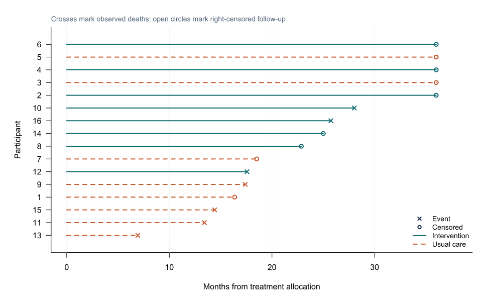
Each horizontal line begins at the common time origin.

A death mark means the event time is observed.

A censor mark means the participant was event free until that time, after which their event time is unknown.

Independent censoring

Kaplan–Meier and Cox methods require censoring to be non-informative under the model.

Informally, participants censored at a time should have a future event prognosis comparable with those remaining under observation, conditional on included information.

Administrative censoring is often plausible.

Loss caused by worsening illness may violate the assumption.

Possible responses include:

• collecting complete follow-up;
• including prognostic variables;
• inverse-probability-of-censoring weighting;
• sensitivity analysis;
• joint modelling.

Interpreting the endpoint

Presenting the results

Suggested reporting

State the time origin, event, censoring rule, follow-up period, event count, number censored, delayed-entry handling and competing-event strategy.

Foundational survival-analysis texts distinguish the event process, censoring process and risk set explicitly [2], [3].

Common mistakes

Knowledge check

What does right censoring mean?

Answer and reasoning

The participant is known to be event free up to the censoring time, but the exact later event time is unknown.

Is the hazard a probability?

Answer and reasoning

No. It is an instantaneous event rate among participants still at risk.

Why must the time origin be defined?

Answer and reasoning

The same event can produce different survival times and risk sets under different origins.

How should delayed entry be represented?

Answer and reasoning

The participant enters the risk set at the observed entry time using a start–stop survival representation.

Does administrative censoring mean the participant survived forever?

Answer and reasoning

No. It means the participant was event free through the administrative censoring time.

Key take-home messages

References

1. Therneau TM. A package for survival analysis in R. R package survival version 3.8-9. 2026. https://CRAN.R-project.org/package=survival
2. Klein JP, Moeschberger ML. Survival analysis: techniques for censored and truncated data. 2nd ed. New York: Springer; 2003. https://doi.org/10.1007/b97377
3. Kalbfleisch JD, Prentice RL. The statistical analysis of failure time data. 2nd ed. Hoboken (NJ): Wiley; 2002. https://doi.org/10.1002/9781118032985