Repeated Binary and Count Outcomes

Overview

Repeated outcomes are not always numerical.

Common longitudinal outcomes include:

• binary: controlled or uncontrolled;
• count: hospital visits, falls or infections;
• ordinal: symptom grade;
• nominal: disease state.

The correlation and outcome distribution must both be represented.

Common approaches include:

• marginal GEE;
• generalised linear mixed models;
• transition models;
• multistate models;
• recurrent-event methods.

This lecture focuses on repeated binary and count outcomes.

Why this matters

Applying ordinary logistic or Poisson regression to every repeated row assumes independence.

Consequences include incorrect standard errors and misleading interpretation.

For non-Gaussian outcomes, GEE and mixed models also produce different coefficient meanings:

• GEE: population-averaged effect;
• GLMM: cluster- or subject-specific conditional effect.

The numerical values can differ even when both models are valid [1].

When to use this method

Use a repeated binary or count model when one participant contributes several non-Gaussian outcomes.

Choose the model from:

• outcome distribution;
• population-averaged or subject-specific estimand;
• visit timing;
• correlation structure;
• overdispersion;
• zero process;
• missingness.

Research question and variables

Binary model:

$$\log\left[ \frac{P(Y_{ij}=1)} {1-P(Y_{ij}=1)} \right] = \beta_0+\beta_1G_i+\beta_2t_{ij} +\beta_3G_it_{ij}+\beta_4A_i$$

Count model:

$$\log E(C_{ij}) = \gamma_0+\gamma_1G_i+\gamma_2t_{ij} +\gamma_3G_it_{ij}+\gamma_4A_i$$

Time is coded as visit index 0, 1 and 2, representing three-month steps.

Data structure

Repeated binary and count outcomes

simulated data

Table 1. Observed group summaries

Outcome	Group	Baseline	Month 3	Month 6
Controlled, %	Usual care	35.0	40.0	36.7
Controlled, %	Telemonitoring	40.0	58.3	80.0
Mean visit count	Usual care	1.02	1.55	1.62
Mean visit count	Telemonitoring	1.15	0.73	1.18

Note: Values are deterministic simulated outcomes.

Statistical assumptions

Generating the simulated outcomes

The R code creates deterministic outcomes so the lecture can be reproduced exactly.

make_longitudinal_data <- function(n = 120) {
  records <- vector("list", n * 3)
  row_number <- 1

  for (participant_id in seq_len(n)) {
    group <- as.integer(participant_id %% 2 == 0)
    age <- 35 + ((7 * participant_id) %% 41)
    male <- as.integer(participant_id %% 3 == 0)

    random_intercept <-
      7 * sin(participant_id * 0.71) +
      3 * cos(participant_id * 0.19)

    random_slope <-
      0.45 * sin(participant_id * 0.37)

    for (month in c(0, 3, 6)) {
      residual <-
        3.5 * sin(participant_id * 1.13 + month * 0.91) +
        1.2 * cos(participant_id * 0.23 + month * 0.33)

      sbp <-
        151 +
        0.18 * (age - 55) +
        1.8 * male +
        random_intercept -
        1.5 * month -
        0.4 * group -
        0.75 * group * month +
        random_slope * month +
        residual

      records[[row_number]] <- data.frame(
        id = participant_id,
        group_numeric = group,
        group = factor(
          group,
          levels = c(0, 1),
          labels = c("Usual care", "Telemonitoring")
        ),
        age = age,
        male = male,
        month = month,
        time_index = match(month, c(0, 3, 6)) - 1,
        sbp = sbp
      )

      row_number <- row_number + 1
    }
  }

  longitudinal <- do.call(rbind, records)
  longitudinal <- longitudinal[
    order(longitudinal$id, longitudinal$month),
  ]
  rownames(longitudinal) <- NULL
  longitudinal
}

longitudinal <- make_longitudinal_data()

longitudinal$logit_probability <-
  -0.7 +
  0.15 * longitudinal$time_index +
  0.25 * longitudinal$group_numeric +
  0.70 * longitudinal$group_numeric *
    longitudinal$time_index -
  0.012 * (longitudinal$age - 55) +
  0.35 * sin(longitudinal$id * 0.29)

longitudinal$probability_controlled <-
  plogis(longitudinal$logit_probability)

deterministic_uniform <-
  (
    (
      longitudinal$id * 37 +
      longitudinal$time_index * 19
    ) %% 100 +
    0.5
  ) / 100

longitudinal$controlled <- as.integer(
  deterministic_uniform <
    longitudinal$probability_controlled
)

subject_multiplier_values <-
  c(0.35, 0.70, 1.00, 1.40, 2.20)

subject_multiplier <-
  subject_multiplier_values[
    ((longitudinal$id * 7) %% 5) + 1
  ]

longitudinal$expected_visits <-
  exp(
    0.15 +
    0.22 * longitudinal$time_index -
    0.18 * longitudinal$group_numeric -
    0.20 * longitudinal$group_numeric *
      longitudinal$time_index +
    0.01 * (longitudinal$age - 55)
  ) *
  subject_multiplier

count_multiplier_values <-
  c(0, 0.6, 1.0, 1.4, 2.0, 0.3)

count_multiplier <-
  count_multiplier_values[
    (
      (
        longitudinal$id * 5 +
        longitudinal$time_index * 3
      ) %% 6
    ) + 1
  ]

longitudinal$visits <- round(
  longitudinal$expected_visits *
    count_multiplier
)

Worked example

The two analyses use the same participants and visit structure but different outcome distributions and link functions.

Repeated binary outcome

A binomial logistic GEE estimates population-average odds ratios.

Repeated count outcome

A Poisson log-link GEE estimates population-average count-mean ratios when observation time is equal.

Worked analysis in R

The geepack package fits both models [2].

library(geepack)

binary_gee <- geeglm(
  controlled ~ group * time_index + age,
  id = id,
  data = longitudinal,
  family = binomial(link = "logit"),
  corstr = "exchangeable",
  std.err = "san.se"
)

count_gee <- geeglm(
  visits ~ group * time_index + age,
  id = id,
  data = longitudinal,
  family = poisson(link = "log"),
  corstr = "exchangeable",
  std.err = "san.se"
)

summary(binary_gee)
summary(count_gee)

binary_output <- coef(summary(binary_gee))
count_output <- coef(summary(count_gee))

exp(
  cbind(
    estimate = coef(binary_gee),
    confint.default(binary_gee)
  )
)

exp(
  cbind(
    estimate = coef(count_gee),
    confint.default(count_gee)
  )
)

Reference binary GEE output for local R verification

Term                         Log OR   Robust SE   OR      95% CI
Telemonitoring at baseline    0.078     0.384     1.08    0.51 to 2.29
Time step                     0.036     0.218     1.04    0.68 to 1.59
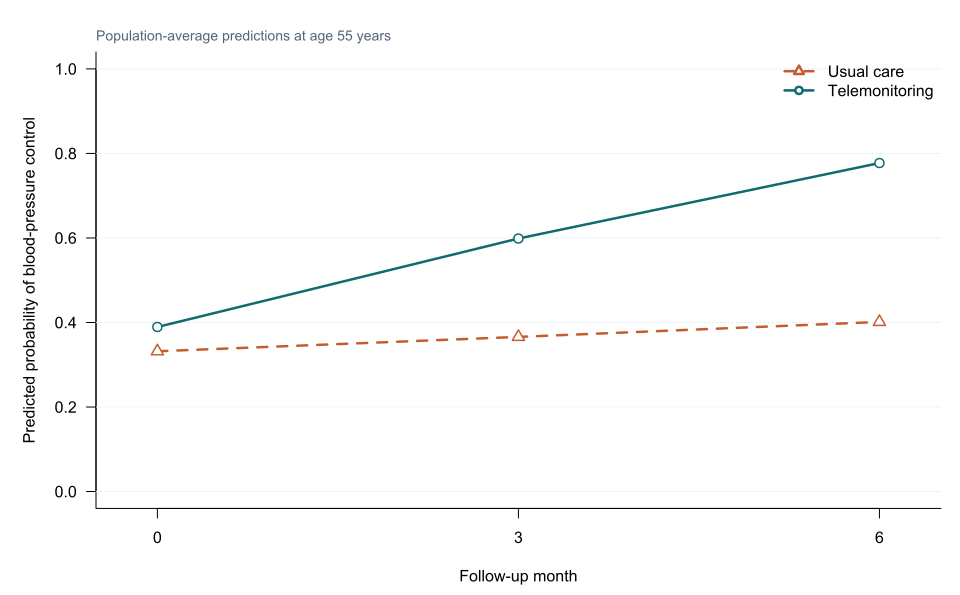
Telemonitoring × time         0.852     0.268     2.34    1.39 to 3.97
Age                          -0.013     0.012     0.987   0.964 to 1.011

Reference count GEE output for local R verification

Term                         Log ratio   Robust SE   Ratio   95% CI
Telemonitoring at baseline     -0.066      0.145      0.936   0.704 to 1.245
Time step                       0.217      0.026      1.242   1.180 to 1.307
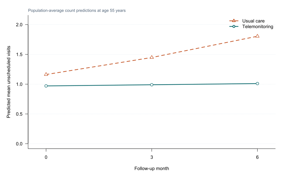
Telemonitoring × time          -0.200      0.028      0.818   0.774 to 0.865
Age                             0.015      0.006      1.015   1.004 to 1.027

Visualising predicted probabilities

Visualising predicted count means

Population-averaged versus subject-specific effects

For binary outcomes, a logistic mixed model includes participant random effects:

glmer(
  controlled ~ group * time_index + age +
    (1 | id),
  data = longitudinal,
  family = binomial
)

Its odds ratios are conditional on the random effect and are usually farther from one than population-average GEE odds ratios.

The two models answer different questions rather than one being universally superior.

Overdispersion and excess zeros

Poisson GEE with sandwich SEs protects selected uncertainty against variance misspecification when the marginal mean is correct and clusters are numerous.

However, the count distribution should still be examined.

For subject-specific modelling with overdispersion, options include:

• negative-binomial GLMM;
• observation-level random effects;
• zero-inflated or hurdle models when scientifically justified.

The glmmTMB package supports several such models [3].

Many zeros do not automatically prove a separate structural-zero process.

Exposure time

If participants contribute unequal observation time, include a log-time offset:

offset(log(person_time))

Without the offset, the model compares counts rather than rates.

Missing outcomes

Binary and count missingness can depend on previous outcomes, hospitalisation or treatment.

Ordinary available-case GEE does not automatically remove missing-data bias. Weighted GEE, multiple imputation or joint models may be required. Likelihood-based repeated-outcome modelling and missing-data assumptions are developed in detail by Fitzmaurice and colleagues [4].

Interpreting the output

Presenting the results

Suggested reporting

Report outcome coding, family, link, cluster identifier, working correlation or random-effects structure, exposure-time offset, robust or model-based variance, overdispersion assessment, missing-data method and marginal predictions [1], [2], [3].

Common mistakes

Knowledge check

What does the binary GEE interaction OR of 2.34 mean?

Answer and reasoning

For each visit step, the telemonitoring-versus-usual-care odds ratio is multiplied by 2.34 on the population-average scale.

Why is that not a risk ratio?

Answer and reasoning

Odds and probabilities use different denominators, especially when the outcome is common.

What does count interaction ratio 0.818 mean?

Answer and reasoning

The telemonitoring-versus-usual-care count ratio is multiplied by 0.818 at each visit step.

When is a person-time offset required?

Answer and reasoning

When participants contribute different observation times and the estimand is an event rate.

Why might a logistic GLMM give a different OR from GEE?

Answer and reasoning

The GLMM estimates a subject-specific conditional effect, whereas GEE estimates a population-average effect.

Key take-home messages

References

1. Zeger SL, Liang KY, Albert PS. Models for longitudinal data: a generalized estimating equation approach. Biometrics. 1988;44(4):1049–1060. https://doi.org/10.2307/2531734
2. Højsgaard S, Halekoh U, Yan J. The R package geepack for generalized estimating equations. J Stat Softw. 2006;15(2):1–11. https://doi.org/10.18637/jss.v015.i02
3. Brooks ME, Kristensen K, van Benthem KJ, Magnusson A, Berg CW, Nielsen A, et al. glmmTMB balances speed and flexibility among packages for zero-inflated generalized linear mixed modeling. R J. 2017;9(2):378–400. https://doi.org/10.32614/RJ-2017-066
4. Fitzmaurice GM, Laird NM, Ware JH. Applied longitudinal analysis. 2nd ed. Hoboken (NJ): Wiley; 2011.