
Part 11 · Module 1
Understanding the Diagnostic 2 × 2 Table
Learn how to construct, label and interpret the diagnostic 2 × 2 table by separating index-test results from target-condition status.
Learning outcomes
After completing this lecture, you should be able to:
- Define the index test, reference standard and target condition.
- Construct a correctly oriented diagnostic 2 × 2 table.
- Identify true-positive, false-negative, false-positive and true-negative cells.
- Distinguish disease prevalence from test positivity.
- Explain how indeterminate results and missing verification affect the table.
- Use R code to create and validate a diagnostic contingency table.
Overview
The diagnostic 2 × 2 table cross-classifies:
- the index test result;
- the target-condition status determined by a reference standard.
Its four cells are:
- true positive;
- false negative;
- false positive;
- true negative.
Every familiar binary diagnostic-accuracy measure is calculated from these cells [1].
A correct table requires more than arranging four numbers. The analyst must define:
- intended use of the test;
- clinical role;
- target condition;
- index-test positivity;
- reference standard;
- participant spectrum;
- handling of indeterminate and missing results.
STARD 2015 emphasises transparent reporting of these design and analysis features [2], with detailed explanation of how intended use and clinical role shape the required accuracy [3].
Why this matters
A transposed or ambiguously labelled table can reverse sensitivity, specificity or predictive values.
Common errors include:
- putting disease status in the wrong denominator;
- calling reference-positive results “test positive”;
- excluding indeterminate index-test results silently;
- verifying only index-test-positive participants;
- treating an imperfect reference as truth without qualification;
- calculating accuracy from percentages instead of participant counts.
The 2 × 2 table should be reconstructed and checked before any summary measure is reported.
When to use this method
Use a diagnostic 2 × 2 table when:
- the index test has two categories;
- the target condition has two categories;
- every participant has both results;
- one participant contributes once;
- index and reference interpretations are sufficiently blinded and independent.
For continuous tests, the table is specific to one threshold.
For multi-category tests, report the full cross-classification or define clinically justified categories before analysis.
Research question and variables
The index test is Test A.
The target condition is disease = 1.
The positivity rule is:
The 2 × 2 table is:
| Target condition present | Target condition absent | |
|---|---|---|
| Index test positive | TP | FP |
| Index test negative | FN | TN |
This orientation keeps disease-specific denominators in columns and test-result categories in rows.
Data structure
Participant-level diagnostic data
simulated dataTable 1. Required variables
| Variable | Meaning |
|---|---|
id | Participant identifier |
score_a | Continuous index-test measurement |
test_a_positive | Binary index-test classification |
disease | Reference target-condition status |
age, male | Participant characteristics for spectrum analysis |
One row per participant is appropriate when each person receives one index test and one reference classification.
Statistical assumptions
How the table works
The marginal totals are also important:
- diseased total: ;
- non-diseased total: ;
- test-positive total: ;
- test-negative total: ;
- total sample: all four cells.
Worked example
Worked analysis in R
make_diagnostic_data <- function(n = 400) {
  id <- seq_len(n)
  age <- 20 + ((7 * id) %% 61)
  male <- as.integer(id %% 2 == 0)

  disease <- as.integer(
    ((id * 37) %% 100) < 30
  )

  score_a <-
    47 +
    11 * disease +
    0.08 * (age - 50) +
    7.5 * sin(id * 1.13) +
    3.5 * cos(id * 0.37)

  score_b <-
    48 +
    9 * disease +
    0.05 * (age - 50) +
    7.2 * sin(id * 1.13 + 0.45) +
    4.0 * cos(id * 0.37 + 0.20)

  disease_rank <- (id * 43) %% 100
  nondisease_rank <- (id * 47) %% 100

  reference_positive <- ifelse(
    disease == 1,
    disease_rank < 88,
    nondisease_rank >= 95
  )

  data.frame(
    id = id,
    age = age,
    male = male,
    disease = disease,
    score_a = score_a,
    score_b = score_b,
    reference_positive = as.integer(
      reference_positive
    )
  )
}

diagnostic_data <- make_diagnostic_data()

cutoff_a <- 51.962318662698785
cutoff_b <- 55.26626112612387

diagnostic_data$test_a_positive <- as.integer(
  diagnostic_data$score_a >= cutoff_a
)

diagnostic_data$test_b_positive <- as.integer(
  diagnostic_data$score_b >= cutoff_b
)

diagnostic_table <- with(
  diagnostic_data,
  table(
    "Index test" = factor(
      test_a_positive,
      levels = c(1, 0),
      labels = c("Positive", "Negative")
    ),
    "Target condition" = factor(
      disease,
      levels = c(1, 0),
      labels = c("Present", "Absent")
    )
  )
)

diagnostic_table
addmargins(diagnostic_table)

tp <- diagnostic_table["Positive", "Present"]
fp <- diagnostic_table["Positive", "Absent"]
fn <- diagnostic_table["Negative", "Present"]
tn <- diagnostic_table["Negative", "Absent"]
Selected analysis output
             Target condition
Index test   Present  Absent
Positive         101      70
Negative          19     210
The displayed counts can be recalculated from the simulated data using the R code above.
Visualising the 2 × 2 table
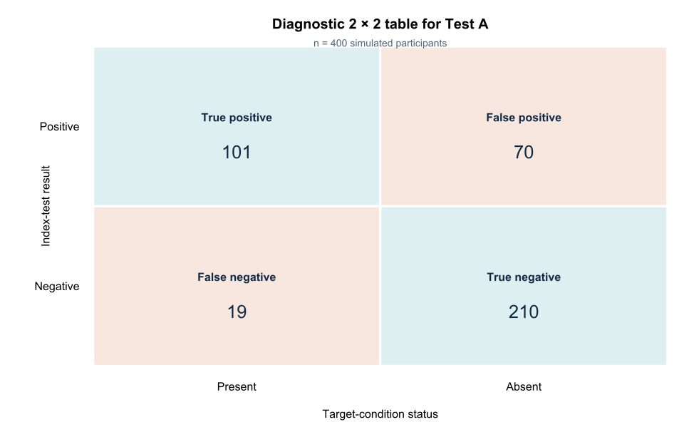
The figure is a learning aid. Manuscripts should usually present a labelled table with counts.
Indeterminate results
An index test may be:
- positive;
- negative;
- indeterminate;
- failed;
- technically inadequate.
Forcing every indeterminate result into positive or negative can distort accuracy.
Report:
- number indeterminate;
- reason;
- whether repeat testing occurred;
- primary handling;
- sensitivity analyses.
STARD asks authors to explain how indeterminate index-test or reference results were handled [2].
Partial verification
Verification bias occurs when only selected participants receive the reference standard.
For example, confirming disease only after a positive index test can:
- overestimate sensitivity;
- underestimate false negatives;
- distort predictive values.
The participant flow should show who received each test.
Spectrum and setting
Accuracy is not a fixed intrinsic property.
It can vary with:
- disease severity;
- alternative diagnoses;
- referral setting;
- prior testing;
- demographic characteristics;
- technical execution.
A case–control sample of clearly diseased cases and healthy controls may yield optimistic separation compared with a consecutive clinical population. Diagnostic-study design and analysis are developed in detail by Zhou and colleagues [4].
Interpreting the output
Presenting the results
Suggested reporting
Report recruitment method, clinical setting, participant spectrum, index and reference procedures, thresholds, blinding, time interval, indeterminate results and the complete 2 × 2 table [2], [3].
Common mistakes
Knowledge check
Which cells contain participants with the target condition?
Answer and reasoning
True-positive and false-negative cells.
What is the denominator for disease prevalence?
Answer and reasoning
All participants in the relevant study sample.
Why is test positivity not prevalence?
Answer and reasoning
Test positivity includes true positives and false positives, whereas prevalence is defined by reference target-condition status.
What is partial verification bias?
Answer and reasoning
Only a selected subset receives the reference standard, often depending on the index-test result.
Why must the threshold be stated?
Answer and reasoning
The 2 × 2 table and all threshold-dependent accuracy measures change when the cut-off changes.
Key take-home messages
References
- Altman DG, Bland JM. Diagnostic tests 1: sensitivity and specificity. BMJ. 1994;308(6943):1552. https://doi.org/10.1136/bmj.308.6943.1552
- Bossuyt PM, Reitsma JB, Bruns DE, Gatsonis CA, Glasziou PP, Irwig L, et al. STARD 2015: an updated list of essential items for reporting diagnostic accuracy studies. BMJ. 2015;351:h5527. https://doi.org/10.1136/bmj.h5527
- Cohen JF, Korevaar DA, Altman DG, Bruns DE, Gatsonis CA, Hooft L, et al. STARD 2015 guidelines for reporting diagnostic accuracy studies: explanation and elaboration. BMJ Open. 2016;6:e012799. https://doi.org/10.1136/bmjopen-2016-012799
- Zhou XH, Obuchowski NA, McClish DK. Statistical methods in diagnostic medicine. 2nd ed. Hoboken (NJ): Wiley; 2011. https://doi.org/10.1002/9780470906514
These notes support learning and research planning and do not replace statistical consultation for a specific study.