Mixed-Effects Models

Overview

Mixed-effects models combine:

• fixed effects, which describe population-level mean relations;
• random effects, which represent variation among participants, clinics or other grouping units.

For longitudinal numerical outcomes, a linear mixed model can represent repeated observations using a participant-specific random intercept, random slope or both.

The model provides subject-specific conditional predictions and estimates variance components explicitly.

Random-effects models for longitudinal data were formalised by Laird and Ware [1].

Why this matters

Participants can begin at different outcome levels and can change at different rates.

A population mean profile alone does not describe this heterogeneity.

Mixed-effects models can:

• separate between-participant and within-participant variation;
• estimate population fixed effects;
• estimate participant-specific deviations;
• handle unequal observation numbers under likelihood assumptions;
• represent several hierarchical levels.

They do not automatically provide unbiased results under arbitrary missingness or model misspecification.

When to use this method

Use a mixed-effects model when:

• observations are nested within participants or clusters;
• subject-specific heterogeneity is scientifically meaningful;
• participant-specific predictions are useful;
• incomplete or irregular repeated data must be represented;
• several hierarchical levels exist.

Choose random effects from the design and scientific question rather than automated significance testing alone.

Research question and variables

The random-intercept model is:

The group-by-month fixed effect describes the average difference in slopes.

Data structure

Mixed-model levels

simulated data

Table 1. Hierarchical structure

Level	Unit	Variables
Level 2	Participant	Group, age, sex, random intercept
Level 1	Visit	Month, systolic blood pressure, residual

A participant-level predictor cannot vary across that participant’s rows unless the data are incorrect.

Statistical assumptions

Random intercepts and slopes

Random intercept

Allows each participant to have a different baseline level while sharing the same fixed slope.

Random slope

Allows each participant to have a different change rate.

A random-intercept-and-slope model is:

$$Y_{ij} = \text{fixed part} + b_{0i} + b_{1i}t_{ij} + \varepsilon_{ij}$$

The random intercept and slope can be correlated.

A complex random structure with only three visits can be difficult to estimate. Singular fits indicate that one or more variance components are estimated near the boundary.

How the method works

Mixed models use maximum likelihood or restricted maximum likelihood.

Restricted maximum likelihood

REML is commonly used to estimate variance components in a fixed model.

Maximum likelihood

ML is generally used when comparing nested models that differ in fixed effects.

Models with different fixed effects should not be compared using REML likelihoods.

Conditional and marginal means

The fixed-only prediction is the population mean conditional on covariates.

Adding a participant’s random effect gives a subject-specific fitted trajectory.

Random-effect estimates are shrunken towards zero, especially for participants with little information.

Worked example

Worked analysis in R

The lme4 package implements linear mixed models, and lmerTest provides Satterthwaite approximations for fixed-effect tests [2], [3].

make_longitudinal_data <- function(n = 120) {
  records <- vector("list", n * 3)
  row_number <- 1

  for (participant_id in seq_len(n)) {
    group <- as.integer(participant_id %% 2 == 0)
    age <- 35 + ((7 * participant_id) %% 41)
    male <- as.integer(participant_id %% 3 == 0)

    random_intercept <-
      7 * sin(participant_id * 0.71) +
      3 * cos(participant_id * 0.19)

    random_slope <-
      0.45 * sin(participant_id * 0.37)

    for (month in c(0, 3, 6)) {
      residual <-
        3.5 * sin(participant_id * 1.13 + month * 0.91) +
        1.2 * cos(participant_id * 0.23 + month * 0.33)

      sbp <-
        151 +
        0.18 * (age - 55) +
        1.8 * male +
        random_intercept -
        1.5 * month -
        0.4 * group -
        0.75 * group * month +
        random_slope * month +
        residual

      records[[row_number]] <- data.frame(
        id = participant_id,
        group_numeric = group,
        group = factor(
          group,
          levels = c(0, 1),
          labels = c("Usual care", "Telemonitoring")
        ),
        age = age,
        male = male,
        month = month,
        time_index = match(month, c(0, 3, 6)) - 1,
        sbp = sbp
      )

      row_number <- row_number + 1
    }
  }

  longitudinal <- do.call(rbind, records)
  longitudinal <- longitudinal[
    order(longitudinal$id, longitudinal$month),
  ]
  rownames(longitudinal) <- NULL
  longitudinal
}

longitudinal <- make_longitudinal_data()

library(lme4)
library(lmerTest)

mixed_fit <- lmer(
  sbp ~ group * month + age + male + (1 | id),
  data = longitudinal,
  REML = TRUE
)

summary(mixed_fit)

fixed_effect_ci <- confint(
  mixed_fit,
  parm = "beta_",
  method = "Wald"
)

variance_components <- as.data.frame(
  VarCorr(mixed_fit)
)

participant_variance <- variance_components[
  variance_components$grp == "id",
  "vcov"
]

residual_variance <- sigma(mixed_fit)^2

icc <- participant_variance /
  (participant_variance + residual_variance)

icc

Selected analysis output

Fixed effect                 Estimate   SE       95% CI
Telemonitoring at baseline    -0.542    1.111    -2.720 to 1.637
Month                         -1.519    0.096    -1.707 to -1.331
Telemonitoring × month        -0.737    0.136    -1.003 to -0.471
Age                            0.188    0.044     0.101 to 0.274
Male versus female             1.588    1.094    -0.556 to 3.732

Random-intercept variance = 28.565
Residual variance = 9.951
ICC = 0.742

Small differences may occur because denominator-degree-of-freedom and optimisation procedures vary across software.

Visualising subject-specific fits

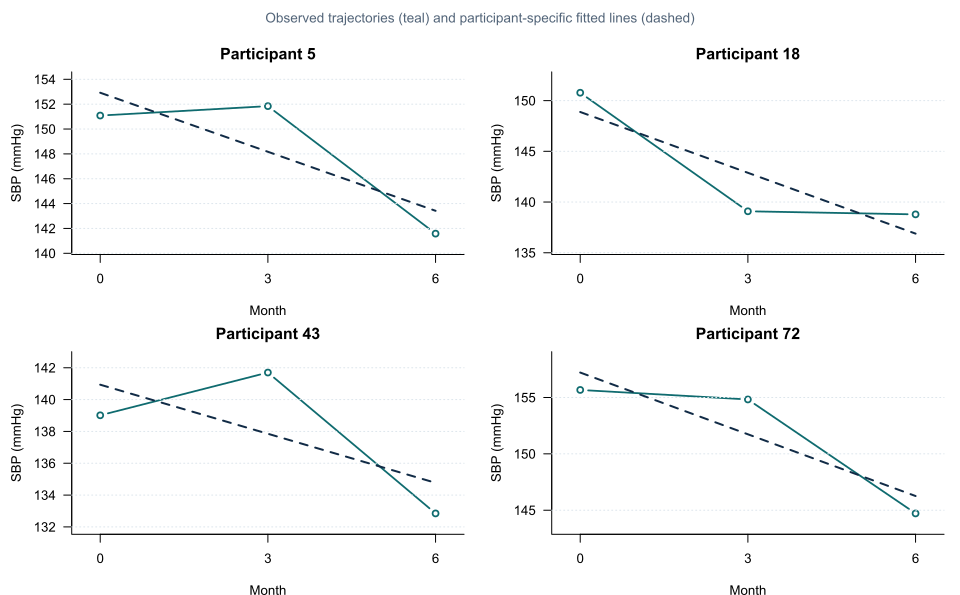
The figure shows selected participants only. Plotting every participant with labels can become unreadable.

Random-effects interpretation

Random effects are not ordinary observed participant characteristics.

They are latent deviations estimated under a distribution and shrunk according to available information.

A caterpillar plot can display participant random intercepts with uncertainty, but it should not be used to rank participants as though their true effects were known exactly.

Missing data

Likelihood-based mixed models can use participants with incomplete outcome vectors under a correctly specified model and a missing-at-random assumption conditional on included information.

They do not solve:

• informative dropout related to unobserved outcomes;
• missing covariates automatically;
• measurement error;
• model misspecification.

Sensitivity analysis remains important. These likelihood and missing-data assumptions are developed in detail in applied longitudinal-analysis frameworks [4].

Interpreting the output

Presenting the results

Suggested reporting

Report fixed effects, random-effects structure, covariance assumptions, estimation method, convergence, singularity, variance components, cluster count, missing-data handling and contrast interpretation [1], [2].

Common mistakes

Knowledge check

What does a random intercept allow?

Answer and reasoning

Each participant can have a different modelled baseline level while sharing the fixed slope structure.

When is ML preferred over REML?

Answer and reasoning

When comparing nested models that differ in fixed effects.

What does ICC 0.742 mean here?

Answer and reasoning

About 74% of residual variance under the random-intercept model is between participants.

What is shrinkage of random effects?

Answer and reasoning

Participant deviations are pulled towards the population mean, particularly when participant information is limited.

Does a random-intercept model allow participant slopes to differ?

Answer and reasoning

No. A random-slope term is needed to model participant-specific change rates.

Key take-home messages

References

1. Laird NM, Ware JH. Random-effects models for longitudinal data. Biometrics. 1982;38(4):963–974. https://doi.org/10.2307/2529876
2. Bates D, Mächler M, Bolker B, Walker S. Fitting linear mixed-effects models using lme4. J Stat Softw. 2015;67(1):1–48. https://doi.org/10.18637/jss.v067.i01
3. Kuznetsova A, Brockhoff PB, Christensen RHB. lmerTest package: tests in linear mixed effects models. J Stat Softw. 2017;82(13):1–26. https://doi.org/10.18637/jss.v082.i13
4. Fitzmaurice GM, Laird NM, Ware JH. Applied longitudinal analysis. 2nd ed. Hoboken (NJ): Wiley; 2011.