Ordinal Logistic Regression

Overview

Ordinal logistic regression models an outcome whose categories have a meaningful order but unknown spacing.

Examples include:

• none, mild, moderate and severe;
• functional class I to IV;
• no improvement, slight improvement and major improvement.

The proportional-odds model estimates one common predictor effect across cumulative category thresholds [1].

Why this matters

Dichotomising an ordinal outcome discards information and makes conclusions depend on a chosen threshold.

Treating category codes as continuous assumes equal spacing that may not exist.

Ordinal regression preserves the category order while avoiding that spacing assumption.

When to use this method

Use ordinal logistic regression when:

• the outcome categories are ordered;
• one category is observed per independent participant;
• cumulative odds are clinically meaningful;
• and the proportional-odds assumption is sufficiently reasonable.

Use multinomial regression when order is absent or when no suitable ordinal structure applies.

Research question and variables

Data structure

Simulated severity distribution

simulated data

Severity	Count
None	63
Mild	61
Moderate	38
Severe	18

The factor level order must be defined explicitly in R.

Statistical assumptions

How the method works

The model estimates threshold intercepts and one slope per predictor.

Exponentiating a slope gives the common odds ratio for being in a higher category across all thresholds.

Understanding cumulative thresholds

For four categories, the model contains three cumulative thresholds. Each threshold divides the outcome into lower versus higher categories.

The threshold intercepts describe the baseline cumulative distribution when predictors equal their reference values. They are necessary for prediction but are rarely reported as clinical effects.

Direction of the model

Software packages use different signs and cumulative-probability conventions. The analyst must verify whether a positive coefficient represents higher or lower categories.

A practical check is to calculate predicted probabilities for two simple profiles. The direction of probability movement should agree with the intended coefficient interpretation.

Assessing proportional odds

The proportional-odds assumption states that one predictor slope applies across all cumulative thresholds. Assessment can include:

• threshold-specific binary logistic estimates;
• graphical comparisons of cumulative logits;
• score or likelihood-based tests;
• clinical consideration of whether one common effect is plausible.

A formal test can reject trivial departures in a large sample or fail to detect important departures in a small sample. Report the threshold pattern rather than relying on one test.

Predicted category probabilities

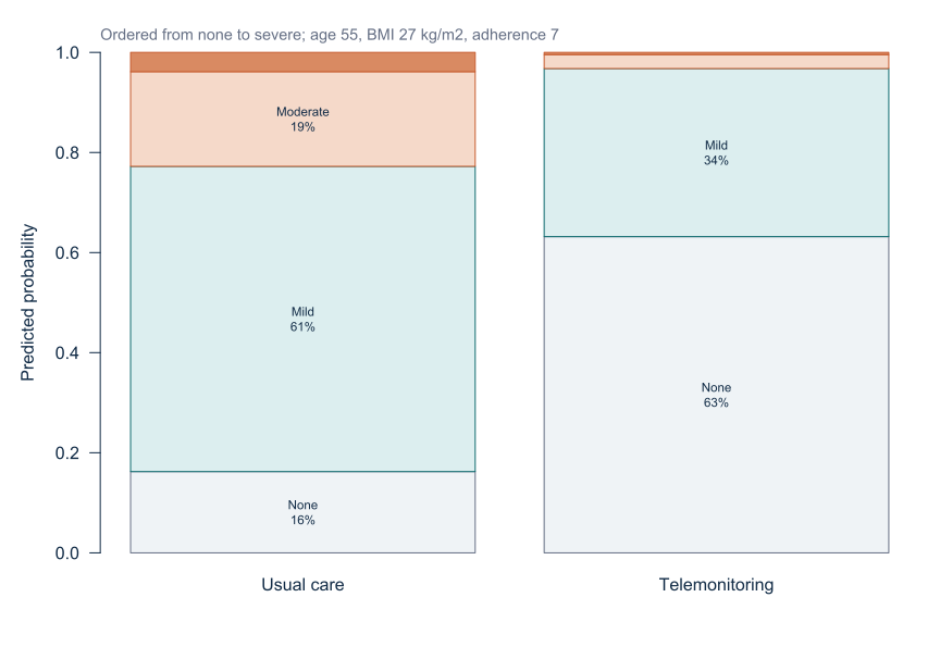
The common odds ratio does not describe the absolute probability of any one category. Predicted probabilities show how the entire distribution shifts.

For communication, report probabilities for clinically meaningful profiles or standardise over the study population. A stacked bar chart can show all category probabilities while preserving the total of 100%.

Partial proportional odds

A partial proportional-odds model allows selected predictors to vary across thresholds while retaining common effects for others. It balances parsimony and flexibility but requires careful coefficient labelling.

When nearly every predictor violates proportional odds, a multinomial or another ordinal structure may be clearer.

Adjacent and continuation-ratio models

Adjacent-category models compare neighbouring categories. Continuation-ratio models represent sequential progression, such as advancing to the next disease stage conditional on reaching the current stage.

These models answer different clinical questions from cumulative proportional odds. Selection should follow the outcome-generating process rather than a search for the smallest p-value.

Repeated ordinal outcomes

Repeated severity ratings from the same participant are correlated. Ordinary polr() assumes independent observations and is unsuitable without a dependence-aware extension.

Possible approaches include ordinal generalised estimating equations, mixed-effects ordinal models or transition models, depending on the population-average or participant-specific estimand.

Worked example

Reproducible R analysis

make_hypertension_data <- function(n = 180) {
  set.seed(4583)
  i <- seq_len(n)

  data <- data.frame(
    participant_id = sprintf("H%03d", i),
    age = round(runif(n, 30, 80)),
    male = rbinom(n, 1, 0.5),
    bmi = pmin(pmax(round(rnorm(n, 27, 3.5), 1), 18), 40),
    physical_activity = round(runif(n, 2, 7), 1),
    telemonitoring = rbinom(n, 1, 0.5)
  )

  data$adherence <- 4 + runif(n, 0, 5) -
    0.015 * (data$age - 55) + 0.4 * data$telemonitoring
  data$baseline_sbp <- 92 + 0.52 * data$age + 0.85 * data$bmi +
    2.8 * data$male - 1.3 * data$physical_activity + rnorm(n, 0, 4)
  data$followup_sbp <- 58 + 0.47 * data$baseline_sbp +
    0.10 * data$age + 0.52 * data$bmi - 2.0 * data$adherence +
    2.0 * data$male - 4.5 * data$telemonitoring -
    0.55 * data$telemonitoring * (data$bmi - 27) +
    0.006 * (data$age - 55)^2 + rnorm(n, 0, 5)

  data
}

hypertension <- make_hypertension_data()

i <- seq_len(nrow(hypertension))

latent_severity <-
  0.035 * (hypertension$age - 55) +
  0.14 * (hypertension$bmi - 27) -
  0.75 * hypertension$telemonitoring -
  0.28 * (hypertension$adherence - 6) +
  0.9 * sin(i * 0.83)

hypertension$severity <- cut(
  latent_severity,
  breaks = c(-Inf, -0.8, 0.2, 1.0, Inf),
  labels = c("None", "Mild", "Moderate", "Severe"),
  ordered_result = TRUE
)

fit <- MASS::polr(
  severity ~ telemonitoring + age + bmi + adherence,
  data = hypertension,
  method = "logistic",
  Hess = TRUE
)

summary(fit)

coefficient_table <- coef(summary(fit))
slopes <- coefficient_table[
  c("telemonitoring", "age", "bmi", "adherence"),
  ,
  drop = FALSE
]

odds_ratios <- exp(slopes[, "Value"])
or_intervals <- exp(
  cbind(
    slopes[, "Value"] - 1.96 * slopes[, "Std. Error"],
    slopes[, "Value"] + 1.96 * slopes[, "Std. Error"]
  )
)

odds_ratios
or_intervals

Cleaned R output

Predictor        Common cumulative OR   95% CI
Telemonitoring          0.113            0.056 to 0.229
Age                     1.072            1.047 to 1.098
BMI                     1.357            1.227 to 1.500
Adherence               0.455            0.348 to 0.594

The recommended MASS package provides polr() for proportional-odds regression [2], [3].

Interpreting the output

Presenting the results

Present the ordered category distribution, common cumulative odds ratios and clinically interpretable predicted probabilities.

Visualising predicted severity

Suggested reporting

When proportional odds fails MMed extension

If effects vary importantly across thresholds, consider partial proportional-odds, adjacent-category, continuation-ratio or multinomial models. These alternatives and their assumptions are developed in authoritative ordinal-data texts [4]. More flexible models require more parameters and adequate category counts.

Common mistakes

Knowledge check

Why is severity ordinal?

Answer and reasoning

Its categories have a meaningful order, but adjacent category distances are not known to be equal.

What does OR = 0.113 mean?

Answer and reasoning

Telemonitoring is associated with lower odds of being in a higher severity category across cumulative thresholds.

Does the odds ratio describe severe versus none only?

Answer and reasoning

No. It is a common cumulative contrast under proportional odds.

Why assess proportional odds?

Answer and reasoning

One common coefficient is inadequate if predictor effects differ substantially across thresholds.

Why report category probabilities?

Answer and reasoning

They show absolute clinical distributions that an odds ratio alone cannot convey.

Key take-home messages

References

1. McCullagh P. Regression models for ordinal data. J R Stat Soc Series B Stat Methodol. 1980;42(2):109–127. https://doi.org/10.1111/j.2517-6161.1980.tb01109.x
2. Venables WN, Ripley BD. Modern applied statistics with S. 4th ed. New York: Springer; 2002. https://doi.org/10.1007/978-0-387-21706-2
3. Ripley B, Venables B. MASS: support functions and datasets for Venables and Ripley’s MASS. R package version 7.3-66. 2026. https://doi.org/10.32614/CRAN.package.MASS
4. Agresti A. Analysis of ordinal categorical data. 2nd ed. Hoboken (NJ): Wiley; 2010. https://doi.org/10.1002/9780470594001