
Part 7 · Module 7
Measures of Epidemiological Association
Learn how to calculate and interpret risk difference, risk ratio, odds ratio, rate ratio and attributable measures using reproducible R code.
Learning outcomes
After completing this lecture, you should be able to:
- Distinguish absolute and relative measures of epidemiological association.
- Calculate risk difference, risk ratio and odds ratio from a cohort two-by-two table.
- Calculate an incidence-rate ratio from events and person-time.
- Interpret attributable fractions without overstating causality.
- Select measures appropriate to cohort, cross-sectional and case-control designs.
- Use reproducible R code to generate effect estimates and confidence intervals.
Overview
Epidemiological association measures compare disease or outcome frequency across exposure groups.
They include:
- risk difference;
- risk ratio;
- prevalence difference;
- prevalence ratio;
- odds ratio;
- incidence-rate difference;
- incidence-rate ratio;
- attributable fraction.
No single measure is universally best; measure selection follows the epidemiological question and design [2].
Absolute measures describe additional outcome burden. Relative measures describe proportional contrast. Clinical and public-health decisions usually benefit from both.
The study design determines which frequencies can be estimated and how confounding, selection and measurement affect interpretation [3]. A case–control study generally cannot estimate population risks directly from sampled case and control counts.
Why this matters
An exposure that doubles risk from 1% to 2% has:
- risk ratio 2.0;
- risk difference 1 percentage point.
An exposure that doubles risk from 20% to 40% has the same risk ratio but a 20-percentage-point risk difference.
Relative effects alone can conceal the absolute burden.
Odds ratios can be especially misleading when interpreted as risk ratios for common outcomes [1].
When to use this method
Use risk measures when:
- a defined population is initially outcome-free or otherwise at risk;
- follow-up is sufficient to classify whether the event occurred;
- and group risks are estimable.
Use prevalence measures in cross-sectional studies of current status.
Use incidence rates when:
- person-time varies;
- events occur over follow-up;
- and the event-count model is appropriate.
Use odds ratios commonly in:
- case–control studies;
- logistic regression;
- contingency-table analyses.
Do not describe an odds ratio as a risk ratio.
Research question and variables
For a cohort two-by-two table:
| Outcome | No outcome | Total | |
|---|---|---|---|
| Exposed | |||
| Unexposed |
The exposed and unexposed risks are:
Data structure
Simulated cohort table
simulated dataTable 1. Outcome by exposure
| Exposure | Outcome | No outcome | Total |
|---|---|---|---|
| Exposed | 60 | 240 | 300 |
| Unexposed | 30 | 270 | 300 |
Note: The table represents a simulated cohort with risks estimable from each exposure group.
Statistical assumptions
How the method works
Risk difference
Risk ratio
Odds ratio
Incidence-rate ratio
If and are event counts and and are person-time:
Attributable fraction among the exposed
Under a causal interpretation:
This quantity describes the fraction of exposed-group risk attributable to exposure only if the comparison represents the counterfactual risk without exposure.
Worked example
Incidence-rate example
The exposed rate is:
or 3.75 events per 100 person-years.
The unexposed rate is:
or 1.67 events per 100 person-years.
The incidence-rate ratio is:
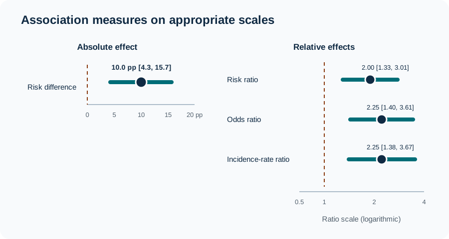
with approximate 95% CI 1.38 to 3.67.
Reproducible R analysis
a <- 60
b <- 240
c <- 30
d <- 270

risk_exposed <- a / (a + b)
risk_unexposed <- c / (c + d)

risk_difference <- risk_exposed - risk_unexposed
risk_ratio <- risk_exposed / risk_unexposed
odds_ratio <- (a * d) / (b * c)

rd_se <- sqrt(
  risk_exposed * (1 - risk_exposed) / (a + b) +
    risk_unexposed * (1 - risk_unexposed) / (c + d)
)
rd_ci <- risk_difference + c(-1, 1) * 1.96 * rd_se

rr_se <- sqrt(
  1 / a - 1 / (a + b) +
    1 / c - 1 / (c + d)
)
rr_ci <- exp(log(risk_ratio) + c(-1, 1) * 1.96 * rr_se)

or_se <- sqrt(1 / a + 1 / b + 1 / c + 1 / d)
or_ci <- exp(log(odds_ratio) + c(-1, 1) * 1.96 * or_se)

nnh <- 1 / risk_difference
af_exposed <- (risk_ratio - 1) / risk_ratio

events_exposed <- 45
pt_exposed <- 1200
events_unexposed <- 25
pt_unexposed <- 1500

rate_exposed <- events_exposed / pt_exposed
rate_unexposed <- events_unexposed / pt_unexposed
rate_ratio <- rate_exposed / rate_unexposed

irr_se <- sqrt(
  1 / events_exposed +
    1 / events_unexposed
)
irr_ci <- exp(log(rate_ratio) + c(-1, 1) * 1.96 * irr_se)

output <- data.frame(
  risk_exposed = risk_exposed,
  risk_unexposed = risk_unexposed,
  risk_difference = risk_difference,
  rd_lower = rd_ci[1],
  rd_upper = rd_ci[2],
  risk_ratio = risk_ratio,
  rr_lower = rr_ci[1],
  rr_upper = rr_ci[2],
  odds_ratio = odds_ratio,
  or_lower = or_ci[1],
  or_upper = or_ci[2],
  nnh = nnh,
  af_exposed = af_exposed,
  rate_ratio = rate_ratio,
  irr_lower = irr_ci[1],
  irr_upper = irr_ci[2]
)

round(output, 3)
Cleaned R output
 risk_exposed risk_unexposed risk_difference rd_lower rd_upper risk_ratio rr_lower rr_upper odds_ratio or_lower or_upper nnh af_exposed rate_ratio irr_lower irr_upper
          0.2            0.1             0.1    0.043    0.157        2.0    1.330    3.007       2.25    1.404    3.606  10        0.5       2.25     1.380     3.668
Interpreting the output
Presenting the results
Table 2. Epidemiological association measures
| Measure | Estimate | 95% CI |
|---|---|---|
| Risk difference | 10.0 percentage points | 4.3 to 15.7 |
| Risk ratio | 2.00 | 1.33 to 3.01 |
| Odds ratio | 2.25 | 1.40 to 3.61 |
| Incidence-rate ratio | 2.25 | 1.38 to 3.67 |
Note: Risk and rate examples use different simulated event counts and denominators.
Suggested reporting
Non-collapsibility and transportability MMed extension
Odds ratios can change after covariate adjustment even when the covariate is not a confounder because the odds ratio is non-collapsible.
Risk differences and risk ratios also vary across populations when baseline risk or effect modification differs.
No effect measure is automatically transportable. Report the target population and clinically relevant absolute risks.
Common mistakes
Knowledge check
What is the difference between risk difference and risk ratio?
Answer and reasoning
Risk difference measures absolute excess probability, while risk ratio compares probabilities multiplicatively.
Why is the odds ratio 2.25 when the risk ratio is 2.00?
Answer and reasoning
Odds and risks use different denominators. With a common outcome, the odds ratio often lies farther from one than the risk ratio.
Can a case–control study estimate the sampled case risk?
Answer and reasoning
No. The case and control numbers are selected by design, so sampled proportions do not represent population risks. The odds ratio remains estimable under suitable assumptions.
What does an incidence-rate ratio compare?
Answer and reasoning
It compares event counts per unit of person-time. It does not directly compare cumulative probabilities over a fixed period.
What is required before interpreting an attributable fraction causally?
Answer and reasoning
The exposed and comparison outcome frequencies must represent suitable counterfactual risks after accounting for confounding, selection, measurement and other biases.
Key take-home messages
References
- Davies HTO, Crombie IK, Tavakoli M. When can odds ratios mislead? BMJ. 1998;316(7136):989–991. https://doi.org/10.1136/bmj.316.7136.989
- Rothman KJ. Epidemiology: an introduction. 2nd ed. New York: Oxford University Press; 2012.
- Lash TL, VanderWeele TJ, Haneuse S, Rothman KJ. Modern epidemiology. 4th ed. Philadelphia: Wolters Kluwer; 2021.
- Agresti A. Categorical data analysis. 3rd ed. Hoboken (NJ): Wiley; 2013.
These notes support learning and research planning and do not replace statistical consultation for a specific study.