Confounding

Overview

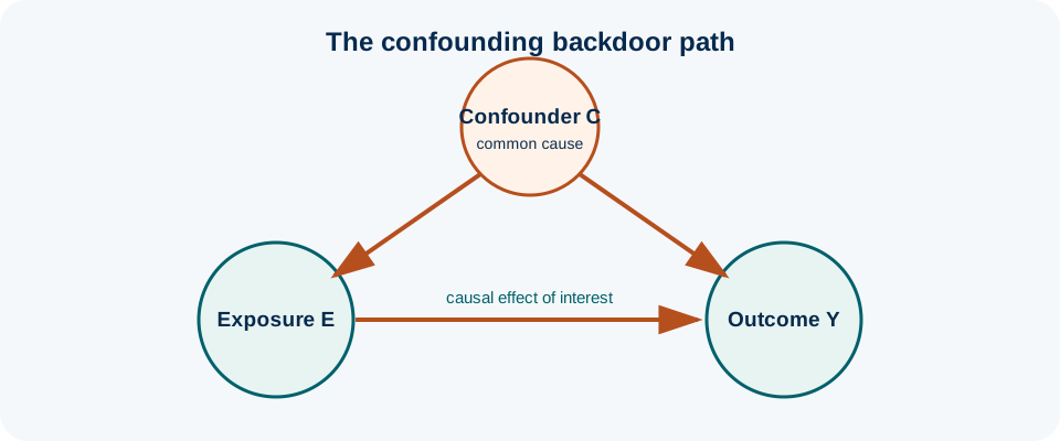
Confounding occurs when the exposure-outcome comparison mixes the effect of the exposure with differences in other causes of the outcome. In causal terms, a confounder is typically a pre-exposure variable, or set of variables, needed to block non-causal pathways between exposure and outcome. Confounding is therefore a property of the causal structure and target effect—not simply a variable that is associated with both exposure and outcome.[1,2]

This distinction matters because statistical association alone is an unreliable method for choosing adjustment variables. Adjusting for a mediator can remove part of the effect being estimated; adjusting for a collider can introduce bias; and failing to measure an important common cause can leave residual confounding.

Why this matters

Confounding is one of the central validity problems in observational health research. People who receive an exposure or treatment often differ from those who do not in prognosis, healthcare access, behaviour or disease severity. If those differences also affect the outcome, a crude comparison can be misleading.

The solution is not to include every available variable in a multivariable model. Modern guidance emphasises defining the causal question first and selecting an adjustment set using prior knowledge of the data-generating process.[1,3]

Key concepts

A variable is not a confounder merely because its inclusion changes an estimate by more than 10%, nor because it has a small p-value in a univariable model. Change-in-estimate rules and significance screening can be unstable and may select inappropriate variables. A more defensible approach uses causal knowledge to identify common causes of exposure and outcome, or uses a principled criterion such as the disjunctive cause approach when the full structure is uncertain.[1]

Effect modification is different: it asks whether the effect itself varies across levels of another variable. Mediation asks whether part of an effect operates through an intermediate variable. These questions require different estimands and analysis strategies.

Time ordering is essential

A confounder must be conceptually prior to the exposure for the total-effect question being asked. Variables measured after exposure can still represent pre-existing characteristics, but researchers must distinguish measurement time from causal time. For example, parity measured at enrolment may predate an intervention; satisfaction measured after the intervention does not.

A variable can also play different roles in different questions. Baseline depressive symptoms may confound the relationship between social support and later depression, yet depression measured after an intervention could be an outcome or mediator.

Causal diagrams and backdoor paths

Directed acyclic graphs (DAGs) make assumed relationships explicit. A backdoor path enters the exposure through an arrow pointing into it and can create a non-causal association with the outcome. An adequate adjustment set blocks relevant backdoor paths without conditioning on descendants of exposure that would alter the estimand or introduce collider bias.[2]

A DAG does not prove that the assumed structure is true. Its value is transparency: reviewers can see why variables were considered confounders and can challenge those assumptions.

Design-stage approaches

Randomisation balances measured and unmeasured baseline causes in expectation and is the strongest design-stage protection against confounding when an experiment is ethical and feasible. Observational designs can use restriction to narrow variation in a confounder or matching to create comparable groups. These methods have costs: restriction limits applicability, and matching variables require appropriate analysis and can make some effects impossible to estimate.

Good measurement of confounders is also a design strategy. A crude binary proxy for socioeconomic position may leave substantial residual confounding even if it is included in the regression model.

Analysis-stage approaches

Common approaches include stratification, standardisation, regression adjustment, matching estimators and propensity-score methods. Each method targets a particular contrast under assumptions such as exchangeability, positivity and correct model specification. The method should be chosen after the estimand and adjustment set are defined.

Propensity scores summarise measured covariate information related to exposure assignment; they do not control unmeasured confounding automatically. Balance diagnostics are more informative than relying on the propensity-model c-statistic.

Overadjustment and collider bias

More adjustment is not always safer. Adjusting for a variable caused by the exposure may estimate a controlled direct effect rather than the total effect, or may induce bias if the mediator-outcome relationship is confounded. Conditioning on a collider can open a non-causal path.

Examples include adjusting for treatment adherence when estimating the effect of randomised assignment, restricting analyses to hospitalised patients when hospitalisation has multiple causes, or adjusting for a post-treatment biomarker without a clearly defined mediation question.

Residual and unmeasured confounding

Residual confounding can persist because a confounder was omitted, measured imprecisely, categorised too crudely or modelled with an incorrect functional form. Even a long list of covariates cannot guarantee exchangeability.

Researchers should identify the most plausible unmeasured confounders and assess whether they could realistically explain the observed association. Negative controls, quantitative bias analysis and E-values are possible sensitivity tools, but none replaces substantive knowledge.[4]

Confounding in routine-care comparisons

Confounding by indication is common when treatment choice responds to disease severity or prognosis. Patients receiving an intensive treatment may appear to have worse outcomes because they were sicker before treatment. Conversely, preventive treatments may be more common among health-conscious patients, creating healthy-user bias.

Active-comparator and new-user designs can improve comparability in pharmacoepidemiology by aligning indication and treatment initiation, but their validity still depends on measured and unmeasured causes.

Reporting confounding control

Report why variables were selected, how they were measured, how continuous variables were modelled, and whether the adjustment set was prespecified. STROBE recommends describing statistical methods used to control confounding and making clear which confounders were adjusted for and why.[5] Avoid presenting a large adjusted model without a causal rationale.

DECISION GUIDE

Build a confounding-control strategy

• Define the exposure, outcome, target effect and time zero.
• List plausible common causes using clinical and epidemiological knowledge.
• Draw a causal diagram when the structure is complex.
• Exclude mediators and colliders from the total-effect adjustment set unless a different estimand is intended.
• Assess positivity, measurement quality and model form for the selected confounders.
• Plan sensitivity analysis for important unmeasured or poorly measured confounding.

Illustrative covariate-role table

illustrative

Table 1. Roles in a postpartum testing study

Variable	Plausible role for total effect of access burden	Adjustment implication
Socioeconomic position	Common cause of burden and testing	Candidate confounder
Distance from clinic	Cause of access burden and testing feasibility	Candidate confounder or component of construct; define carefully
Anxiety after failed appointment	Consequence of access burden	Potential mediator; do not automatically adjust for total effect
Clinic attendance after symptoms	Consequence of symptoms and burden-related access	Potential collider/selection process
Ethnicity	Contextual variable; role depends on causal structure	Do not include solely because it is available

Note: Roles depend on the stated causal question and assumptions.

APPRAISAL CHECKLIST

Questions for appraising confounding

• Was the target effect or causal question stated clearly?
• Were important common causes identified using subject-matter knowledge?
• Were mediators and colliders distinguished from baseline confounders?
• Were confounders measured with sufficient quality and modelled appropriately?
• Was residual or unmeasured confounding addressed in the interpretation or sensitivity analysis?

Minimal sufficient adjustment setsMMed extension

A DAG can contain several valid adjustment sets. A minimal sufficient adjustment set blocks all relevant backdoor paths without containing unnecessary variables. Different valid sets can vary in statistical efficiency and measurement burden. If no measured set blocks all backdoor paths, the causal effect is not identified from the available data without stronger assumptions or external information. This is a design problem, not merely a regression problem.[2]

Positivity, overlap and the limits of adjustment

Successful confounding control requires more than measuring a list of covariates. For each combination of confounders relevant to the target population, there must be a meaningful possibility of receiving each exposure or treatment being compared. This positivity or overlap requirement is easy to violate in clinical data. For example, if almost all patients with severe renal impairment receive one treatment and almost none receive the alternative, the data contain little direct information about the treatment contrast in that subgroup.[3]

Regression adjustment may still produce a coefficient, but the estimate can depend heavily on model extrapolation beyond observed comparisons. Propensity-score methods cannot manufacture overlap either. Investigators should examine the distribution of key confounders and, for propensity-based analyses, the overlap of estimated treatment probabilities. Restricting the target population to a region of common support may improve credibility, but it changes the population to which the estimate applies and should be reported explicitly.

This is an important methodological lesson: a larger dataset does not automatically solve confounding when the comparison itself is structurally absent. Design-stage restriction, choosing an active comparator with similar treatment indications, or redefining the target population may be more defensible than increasingly complex adjustment.

Time-varying confounding

Confounding becomes more difficult when variables change after study entry. Consider a longitudinal treatment study in which disease severity influences subsequent treatment, while prior treatment also affects later disease severity. Current severity is then both a predictor of future treatment and a consequence of earlier treatment. Ordinary adjustment for the latest severity measure can block part of the treatment effect or introduce other bias, whereas failing to account for it leaves confounding of subsequent treatment.[3]

This structure is called time-varying confounding affected by prior exposure. It cannot always be handled correctly by a conventional regression model with time-updated covariates. Methods such as marginal structural models with inverse-probability weighting were developed for settings of this type, provided the relevant treatment and confounding processes are adequately measured.[3]

At the research-methodology stage, the key responsibility is to recognise the structure before analysis. Specify treatment histories, repeated confounder measurements, time origin and causal contrast. If the study only measures confounders once at baseline, no later statistical technique can recover unmeasured time-varying confounding.

Matching does not automatically control confounding

Matching is often described as though it “removes” confounding by design. Its role depends on the design. In case-control studies, matching can improve efficiency or ensure representation across key factors, but the matching variables must be accounted for appropriately in analysis. Matching can also create overmatching, make control selection more difficult and prevent estimation of the effect of an individual matching factor within the matched comparison.[5]

In cohort studies, matching or restriction can improve baseline comparability on selected measured variables, but residual differences may remain. In randomised trials, randomisation—not statistical matching—is the mechanism intended to balance both measured and unmeasured baseline causes on average. These different mechanisms should not be conflated.

The practical question is therefore not “Have we matched?” but “Which causal backdoor paths remain open for the estimand of interest?” A causal diagram and explicit adjustment rationale are usually more informative than a checklist of matching variables.[1,2]

Confounding control for explanation versus prediction

Confounder selection is driven by a causal estimand. Prediction modelling has a different objective: estimating future or unknown outcomes accurately in a target setting. A variable may be an excellent predictor without being a confounder, and a true confounder may contribute little to predictive performance. Selecting variables solely because they are statistically associated with the outcome therefore mixes two different tasks.[1]

For an explanatory or causal study, the adjustment set should be justified by subject-matter knowledge and causal structure, not by automated univariable screening. For a prediction study, variable selection, regularisation and validation should be judged by predictive performance and transportability. Clearly stating which goal the study serves prevents the common error of giving a causal interpretation to a coefficient from a model assembled for prediction.

Interface with statistical analysis

The statistical method—regression, stratification, standardisation, weighting or matching—implements a confounding-control strategy after the adjustment set is chosen. Report the effect estimate on a scale relevant to the research question and assess model diagnostics. The linked Biostatistics content covers adjusted effect estimation; this lecture focuses on why and what to adjust for.

Worked example

WORKED EXAMPLE

From crude association to a defensible adjustment set

A crude analysis suggests women with high access burden have twice the prevalence of incomplete postpartum testing. The team initially proposes adjusting for age, ethnicity, income, distance, employment, parity, baseline HbA1c, anxiety measured at 8 weeks, number of reminder calls and clinic attendance after delivery.

A causal diagram changes the plan. Income, employment flexibility, distance, parity and continuity with primary care are plausible common causes. Anxiety at 8 weeks may be partly caused by repeated access difficulties, making it a potential mediator. Number of reminder calls is a response to missed appointments and should not be treated as a baseline confounder. Postpartum clinic attendance may be affected by both symptoms and access burden, making restriction or adjustment potentially problematic.

The primary model uses a prespecified baseline adjustment set supported by the DAG. A secondary sensitivity analysis adds plausible proxy variables for unmeasured healthcare engagement. The report presents both crude and adjusted estimates and explains why the adjustment set—not the statistical significance of individual covariates—determined the primary model.

Suggested protocol or reporting wording

Common mistakes

Knowledge check

A variable is strongly associated with the exposure but has no causal relationship with the outcome. Is it necessarily a confounder?

Answer and reasoning

No. Association with exposure alone is insufficient. Confounding depends on the causal structure and whether the variable helps block a non-causal path between exposure and outcome.

Why can adjusting for a mediator be inappropriate?

Answer and reasoning

If the target is the total effect, adjusting for a mediator can remove part of the pathway through which the exposure acts and may introduce additional bias. Mediation questions require a separately defined estimand.

Does a propensity score control unmeasured confounding?

Answer and reasoning

No. It balances or adjusts measured variables included in its construction under the chosen method. Unmeasured common causes remain a threat.

What is the value of a DAG if its arrows are assumptions?

Answer and reasoning

It makes causal assumptions explicit, helps distinguish confounders from mediators and colliders, and allows reviewers to identify disputed pathways. Transparency is an advantage even when the graph is uncertain.

Key take-home messages

SUMMARY

Key take-home messages

• Confounding is a causal mixing of effects, not merely a statistical association pattern.
• Choose adjustment variables from the causal question and data-generating structure.
• Mediators, colliders and effect modifiers are not interchangeable with confounders.
• Randomisation, restriction and matching are design-stage strategies; regression and weighting are analysis-stage implementations.
• Residual and unmeasured confounding should be acknowledged and, when important, stress-tested.

References

1. VanderWeele TJ. Principles of confounder selection. Eur J Epidemiol. 2019;34(3):211-219. https://doi.org/10.1007/s10654-019-00494-6
2. Greenland S, Pearl J, Robins JM. Causal diagrams for epidemiologic research. Epidemiology. 1999;10(1):37-48. https://doi.org/10.1097/00001648-199901000-00008
3. Hernán MA, Robins JM. Causal inference: what if. Boca Raton: Chapman & Hall/CRC; 2020. https://www.hsph.harvard.edu/miguel-hernan/causal-inference-book/
4. VanderWeele TJ, Ding P. Sensitivity analysis in observational research: introducing the E-value. Ann Intern Med. 2017;167(4):268-274. https://doi.org/10.7326/M16-2607
5. von Elm E, Altman DG, Egger M, Pocock SJ, Gøtzsche PC, Vandenbroucke JP. The Strengthening the Reporting of Observational Studies in Epidemiology (STROBE) statement. Lancet. 2007;370(9596):1453-1457. https://doi.org/10.1016/S0140-6736(07)61602-X